
Introduction to R for Data Science (Part Three)
This is the third introduction to R. This will cover the basics of data frame, data frame indexing and selection, operations, and more.

PS: Please read ‘Introduction to R for Data Science (Part Two)’ before reading this one. This is a continued version of part two.
Part Two: Introduction to R for Data Science (Part Two)
Data Frames
We will be able to organize and mix data types to create data structures with the help of data frames.
Some built-in data frames (type these in into the console):
state.x77
USPersonalExpenditure
women
WorldPhones
If you want all the data frames available in R use:
data()
If you want to take a peek into the top or bottom data frame use:
head(state.x77)
This would show the first six rows (default).
head(state.x77, 9)
This would show the first nine rows. You can change it to show how many rows you want. If you want to see eleven rows change it to head(state.x77,11). If you want to see four rows change it to head(state.x77,4). You get the idea.
tail(state.x77)
This would show the last six rows.

PS: Ignore the error, I have accidentally written a period instead of a comma.
You can create your own data frames using the data.frame function.
str(dda) would give information about the structure of the data in the data frame.
summary(dda) would give us a summary for each of the columns in our data frame. So we get minimum, median, mean, quartile values, and maximum values.
Data Frames Indexing and Selection
This is how we’re going to grab data out of our data frame.
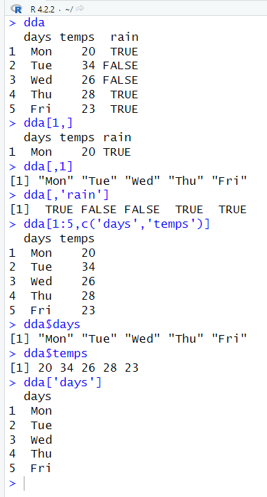
We can use dda[1,] to get the first row back.
We can use dda[,1] to get all the columns from the first row.
We can use dda[,’rain’] to get all the values for rain.
We can use dda[1:5,c(‘days’,’temps’)] to get all the rows, but only the values for days and temps.
We can use dda$days to get all the values for days.
We can do it with temps (dda$temps) and it’ll show all the values for temps
We can use dda[‘days’] to get all the days, but the difference between this one and dda$days is it returns it in a data frame format. If I’m using a dollar sign then I’ll get back a vector.

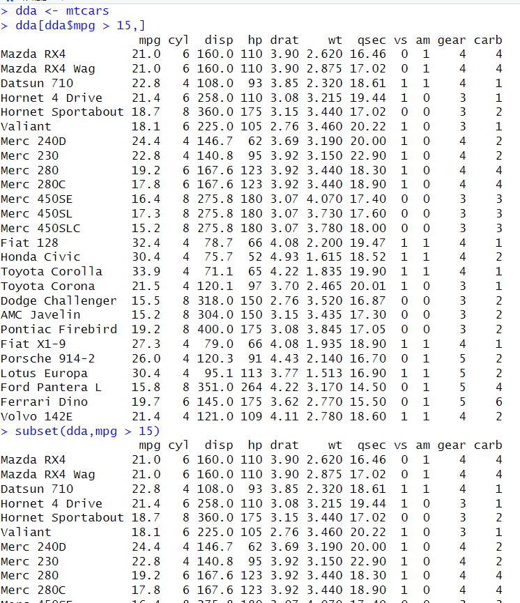
We can use the subset function(subset()) to grab a subset of values from our data. In this case, we want to return rains that are true.
I have also used a subset as a way to get back temperatures greater than 27.

We can also order values from low to high. In this case, I have used order(dda$temps) to order the temperature from low to high.
If we want values from high to low, we would use a negative sign(-) behind the name. So in this case I have used order(-dda$temps) to give me temperatures from high to low.
Data Frame Operations
We’re going to go over operations for the data frame.
Here is a list of basic functions (note that I’m using dda as an example):
nrow(dda)
Will tell you the number of rows
ncol(dda)
Will tell you the number of columns
colnames(dda)
Will tell you the names of columns
rownames(dda)
Will tell you the row names
str(dda)
Will give you the structure of the data
summary(dda)
Will give you the summary of the data

If I wanted a specific value from the table, I would use double brackets. In this case, I wanted to know the value of row three rain. This returns false as row three has rain as false.
You can also change the value by adding a <- ‘value’ after the brackets. In this case, I have changed row two temps to 9394.

If I want to add a new row, I would use rbind(). In this case I have created another frame and have combined them together using rbind(dda,ddb).
If I want to create new columns I can use the dollar sign. In this case, I have created a new column of high temps that is just a multiply of two from temps.
I can also create a copy of days by using dda$copy <- dda$days (not shown above). Note that copy in dda$copy is the column name. You can name it dda$new.copy <- dda$days and it will show the same result, just a different column name.
You can change the names of the columns by using colnames(dda) <- c(‘dddd’, ‘temmm’, ‘rrrraa’) (not shown above). Just add <- after colnames() and the names you want to change it to.
If you want to change a specific column name like if you just want to change column 1 then you can just add [1] after colnames(). If you want to change column 2 name use [2], for column 3 use [3], and so on. For example, colnames(dda)[1] <- ‘New Name’
If you want to check if you have any missing data in your data frame use is.na(). For example, is.na(dda) would give me a FALSE on every value. This shows that there is no missing value. If it is TRUE it means that you’re missing data. You can also use any(is.na()) to check every data in a data frame. For example, any(is.na(dda)) will give me FALSE since I don’t have any missing value. If it outputs TRUE then it shows that I’m missing a value.
Lists
The list is going to help us combine all data structures into a single variable.
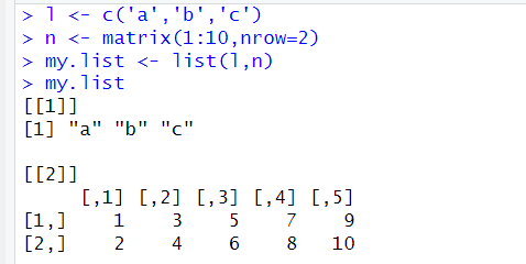
The console is going to display each data structure with double bracket notation ([[1]]). Then the first item on your list.

We can change the double bracket name by adding list(sample.name = l, sample.name2 = n).
You can select a specific object by using a bracket. For example, I would use my.name.list[1] to get the first data structure. You can also use the name that you have given to return the same output. In this case, I can use [‘sample’] to get back the same output.
If you want just the vector and not the name, you can use a $ symbol. You can also use a double bracket to get the same output.
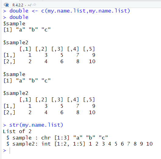
If you want a double list then you can add both lists into a vector.
The best way to get information about a list is by using str(). It’ll tell you how many objects are on the list and what kind of objects they have.
R Programming
I’ll introduce the basics of programming in R.
Logical Operators
Logical operators will help us combine multiple comparison operators.
Here are logical operators:
& (AND)
| (OR)
! (NOT)
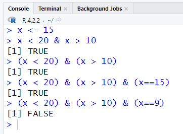
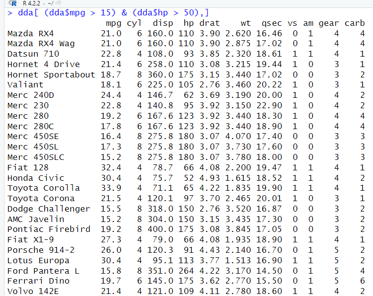
Here I put 15 as the value for x. x is less than 20 and greater than five, which results in true. You can also put parenthesis around it to make it easy to read. You can keep adding and(&) to have more conditions.
If any of the statements are false then it’ll return false.
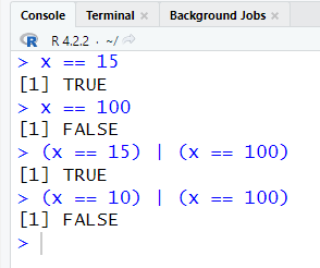
The or operators works by having just one true. In this case, it returns true because one of these statements is true. If one statement isn’t true then it’ll return false.
The not operator works if a value isn’t equal to another value. Here 10 doesn’t equal 1, so it returns true. You can also stack exclamation points together like !!(10 == 1), but you wouldn’t want to do this because it can get messy.
Here are some examples of how you can apply logical operators in your data.
[END of Part Three]