
Introduction to R for Data Science (Part Two)
This is the second introduction to R. This will cover matrix, matrix operations, factor matrices, and more.

PS: Please read ‘Introduction to R for Data Science (Part One)’ before reading this one. This is a continued version of part one.
Part one: Introduction to R for Data Science (Part One)
Vector Indexing and Slicing
We can use bracket notation to index and access individual elements from a vector
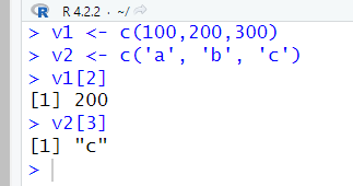
In the figure above, I use v1[2] to select the second number from v1. This would give me 200. I’ve also done it with v2[3] which gave me a “c”. Just remember that if you want to access individual elements, you would use a bracket.
In order to get multiple vectors, we would add a c after the bracket.
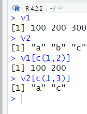
This would allow us to get multiple values as you can see above.
Slicing is where you can grab a continuous slice of vector.
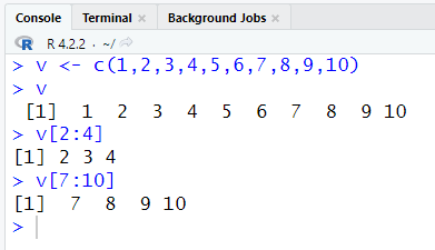
Here I have assigned a new value. The colon(:) is where you would stop. So I would start at 2 and end at 4, which then it gave me 2, 3, and 4. Same thing as v[7:10], it would give me 7, 8, 9, 10.
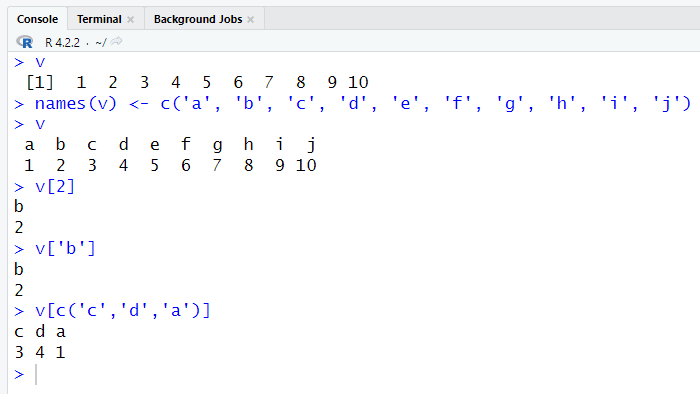
We can also assign characters with numeric as we mentioned before. The difference is that instead of saying v[2], we can also say v[‘b’], which would give us the same result. To get multiple vectors, we can do the same before by using v[c(‘c’,’d’,a’)].
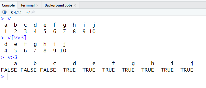
We can also use operators with vectors. So I did v[v>3] which in turn gave me results that are greater than 3.
v>3 would give me a boolean value, so numbers less than three would be false, while numbers above 3 are true.
R Matrices
R matrices are going to allow you to store data.
Creating Matrix
To create a vector fast, we can use 1:10 which would give us 1,2,3,4,5,6,7,8,9,10. We can then assign it to a name. This is just a fast way to create a vector.
To create a matrix, we would use the matrix function which is matrix().
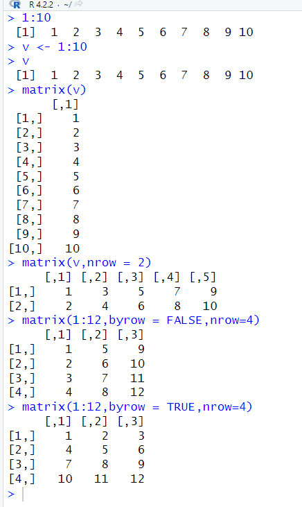
The output of the matrix displays a two-dimensional matrix which is 10 rows by one column.
We can pass a parameter argument into the matrix called nrow, which stands for the number of rows. The output will give us two rows, but because we need to have the correct number of columns in order to equal 10 elements, it is going to give us five columns, since five times two equals 10.
We can use byrow = TRUE to give us a different format of the output.
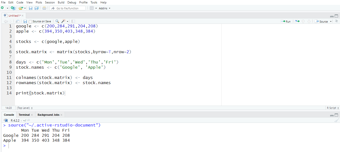
Here is an example of something that you can create.
Note that I’m using an R script (different from the console). You can add a script by clicking on the “paper with a green plus sign” below the files.
Matrix Arithmetic
Here is an example of arithmetic you can use with matrix.
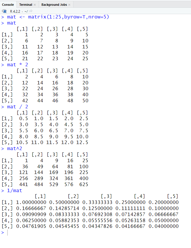
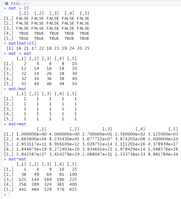
Should be pretty self-explanatory.
Matrix Operations
Some basic functions for Matrix.
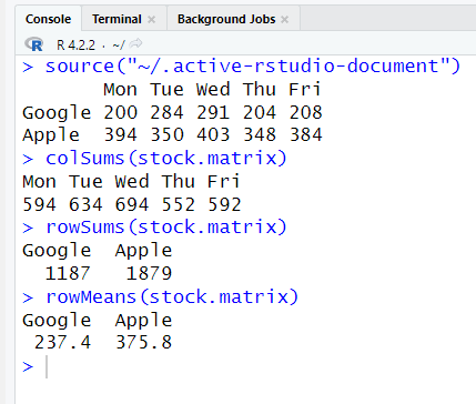
(The values I use are from the Google and Apple stock I have shown you above)
If you want to get the total sum from all the values added, use colSums().
If you want to get the row sums, you can use rowSums().
If you want to get the mean value for rows, use rowMeans().
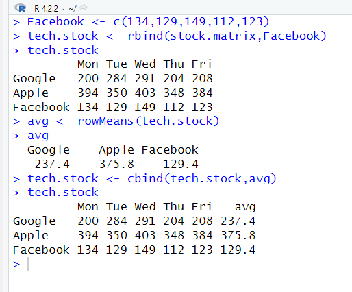
If you want to add another name to your vector, you can use rbind. In this case, I have added Facebook alongside Google and Apple.
If you want to add averages alongside Monday, Tuesday, Wednesday, etc, then you would use rowMeans first, then after which you can use cbind(tech.stock,avg) to add it
Matrix Selection and Indexing
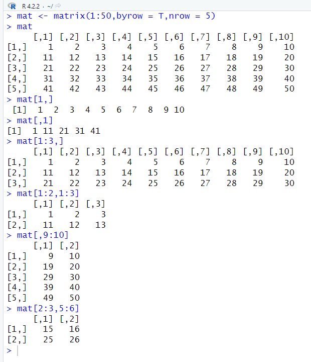
I would use mat[1,] to get all the rows from row one.
I would use mat[,1] to get all the columns from column one.
I would use mat[1:3,] to get all the columns, but only from three rows.
I would use mat[1:2,1:3] to get all the values from column three and row two.
I would use mat[,9:10] to get columns nine and ten.
I would use mat[2:3,5:6] to get a specific value from the table.
Factor and Categorical Matrices
We want to check how many factor levels are in the vector. We can do so by passing the vector through the factor function.
There are going to be nominal categorical variables and ordinal categorical variables. The nominal variables don’t have any order. The ordinal variable has order.
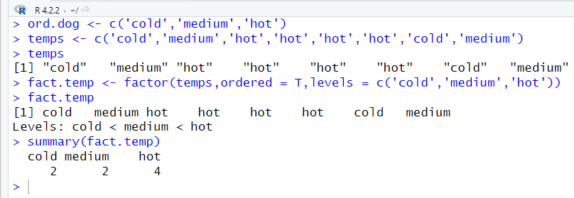
PS: Ignore the ord.dog
In this example, I have created a factor for temperatures. I have used ordered = T to make sure that there is an order from cold to hot.
The levels argument is going to take in a vector and order it the way you want it order. In this case, I want to order it from cold to hot.
The summary function is going to call in a summary on that object. So in this case, I have two cold, two medium, and four hot. Going back on temps there are four hot, two medium, and two cold, so it’s correct.
[End of Part Two]
Part three is coming in four days.