
Introduction to R for Data Science (Part Five)
This is the fifth introduction to R. This would cover apply, math functions, Dplyr, and its features.

PS: Please read ‘Introduction to R for Data Science (Part Four)’ before reading this one. This is a continued version of part four.
Part four: Introduction to R for Data Science (Part Four)
Apply

Using the sample statement is going to randomize a number. It will give us a different number every time you want to run the code.
lapply() is going to take an input function and a vector(can be a list) and it is going to apply this function to every element in the vector. So in a nutshell, it’s saying go to every number and add a random number to it. It will store it as a list.
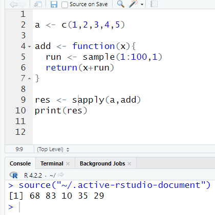
But sometimes, we don’t want a list, so we can use sapply(). This will give us a vector of five(since we have five numbers) with random numbers.
Math Functions
Basic math functions in R:
abs()
sum()
mean()
round()

abs() will give you the absolute value.
sum() will return the sum of all the values.
mean() will give you the mean.
round() will round the decimal. In this case, I want it to round by the second digit, so I put a comma two after the decimal. You can adjust it and put whatever number you want it to round to.
Here is a reference card to have when programming with R: https://cran.r-project.org/doc/contrib/Short-refcard.pdf
Regular Expressions
We’re going to focus on:
grepl()
grep()

grepl() is going to take in the term you’re searching for. In this case, I want to search for “there”. The second thing grepl() will take is the actual thing you want to search which is text in my case. This returns TRUE because ‘there’ is inside the text. If I put something else that isn’t in the text, it will return FALSE.

grep() will return the index location. In this case, I want to know where ‘b’ is, so I’ll use grep() and the results show that it is in the second row. If there was multiple ‘b’ it will show multiple locations like how I did it with ‘c’.
Data Manipulation
Using Dplyr
We’re going to install dplyr. So in order to install it put these steps into your R console:
install.packages(‘dplyr’)
install.packages(‘nycflights13’)
library(dplyr)
library(nycflights13)
Note that nycflights13 is the dataset that I’m going to be using. You can use a different data set if you want.
In order to manipulate data we can use:
filter()
slice()
arrange()
select()
rename()
distinct()
mutate()
transmute()
summarise()
sample_n()
sample_frac

filter() is going to let us filter our data by choosing what we want to filter out of. Here I have filtered all flights that happen on December 5 and specified that the carrier is American Airlines. This gave me all the flights that happen on that date with American Airlines. Note that it didn’t give me all the flights because I have used head(). I’ve used head(), so it doesn’t fill up my screen with data.
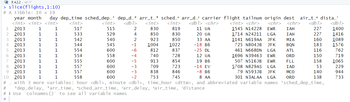
slice() is going to allow you to select rows by positions. In this case, I want the first ten rows, so I put 1:10.

arrange() is going to let us order our data from lowest to highest since this is the default. In this case, I have ordered it by year, month, day, and arr_time. If you want descending order, put desc. I have put descending order on months, so now it shows December first.

select() will allow us to zoom in on a useful subset. It’ll help you gather more data quickly. In this case, it shows me the carrier column since I have selected it. You can also put more rows in like how I put arr_time and months in the second example.

rename() is going to allow you to rename your rows. In this case, I have renamed the carrier into airline_carrier.

distinct() is going to allow us to select the distinct values or unique values in a column. In this case, I have selected carrier and it returns me the unique values. This is similar to the DISTINCT function in SQL.

mutate() will allow us to create another column. In this case, I have created another column of arr_delay - dep_delay. It’s useful when you want to create a formula like how I wanted a column that was based on arrival time minus departure time.
transmute() is similar to mutate(), but with transmute, it only outputs the new column. So mutate will return the entire data set, while transmute will only return the new column you have created.

summarise() will allow us to collapse data frames into single rows using a function that aggregates a result. In this case, I want the mean of the total air_time, so it returns 151. It only returns one row because it’s an aggregate of all the rows. Note that na.rm = TRUE is removing missing data or N/A. There is going to be data that are missing, so we would use na.rm = TRUE. avg_air_time is the name and you can call it whatever you want.
In the second summarise example, I wanted the total time, so I switched out the mean with sum and changed the name to total_time. summarise() is similar to the GROUP BY function in SQL.

sample_n() will give us a random row. In this case, the output is ten random rows.
sample_frac() is similar to sample_n(), but sample_frac is percentage. So if I wanted 10 percent of the rows, I would write 0.1.
[END of Part Five]