
Introduction to R for Data Science (Part Six)
This is the sixth introduction to R. This will cover tidyr, ggplot2, histograms, scatterplots, and more.

PS: Please read ‘Introduction to R for Data Science (Part Five)’ before reading this one. This is a continued version of part five.
Part five: Introduction to R for Data Science (Part Five)
Pipe Operator
The pipe operator is going to allow us to chain together multiple operations.

The pipe operator is just a way to keep things neater. Instead of writing multiple codes, you can just use the pipe operator. In this example I did filter mpg greater than 30, a sample size is four, and had mpg arranged from highest to lowest. Data has to be first, then %>%, and then your operations.
Using Tidyr
Tidyr is going to help us clean data. We’re going to install tidyr. So in order to install it put these steps into your R console:
install.packages('tidyr')
install.packages('data.table')
library(tidyr)
library(data.table)
In order to clean data, we can use:
gather()
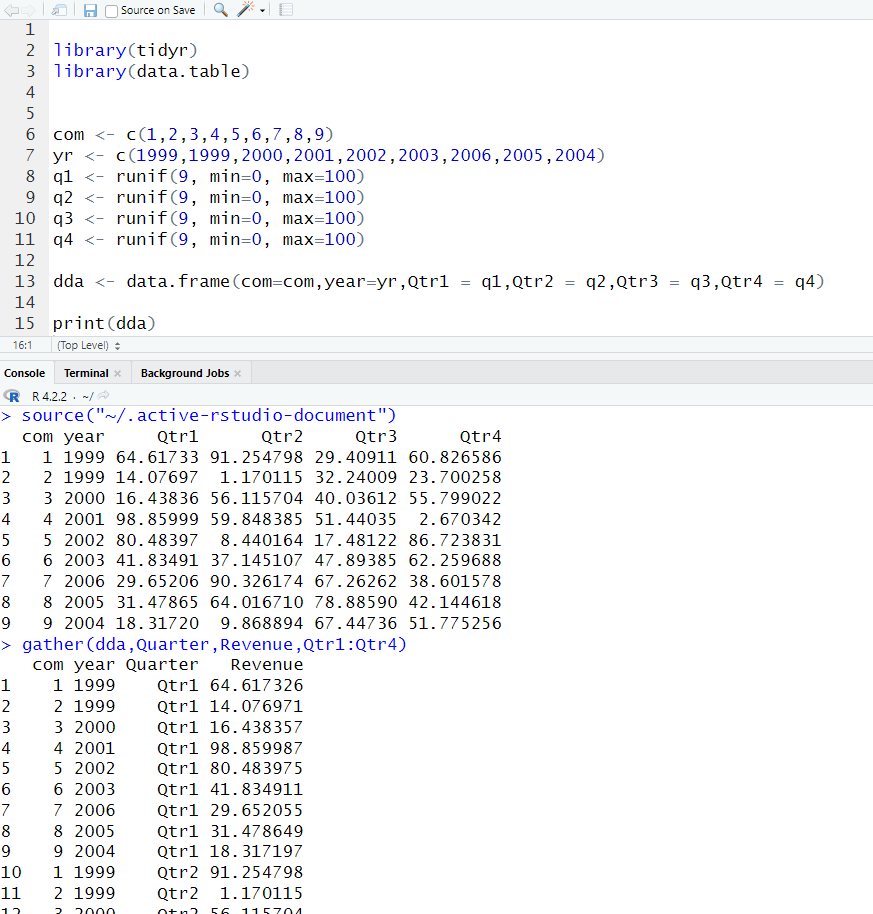
gather() is collapsing Qtr1:Qtr4 into key values which are Quarter and Revenue. This is useful if you want to gather stock prices, and/or quarterly sales data. The Qtr1:Qtr4 is grabbing Qtr1,Qtr2,Qtr3,Qtr4. The revenue is just gathering the data from each quarter.
Data Visualization
ggplot2
ggplot2 follows a distinct philosophy that is built on the idea of adding layers to your visualization.

This article will give you a great explanation of layers: https://englelab.gatech.edu/useRguide/introduction-to-ggplot2.html
Histograms
We’re going to install ggplot2. So in order to install it put these steps into your R console:
install.packages('ggplot2')
install.packages('ggplot2movies')
library(ggplot2)
library(ggplot2movies)
Here is a cheat sheet to make it easier to understand: https://static1.squarespace.com/static/584e336fe3df28e18000d637/t/60ef3aae750ba457d74c3a88/1626290862751/data-visualization-2.1.pdf
Note that ggplot2movies is the dataset that we’re going to work on.
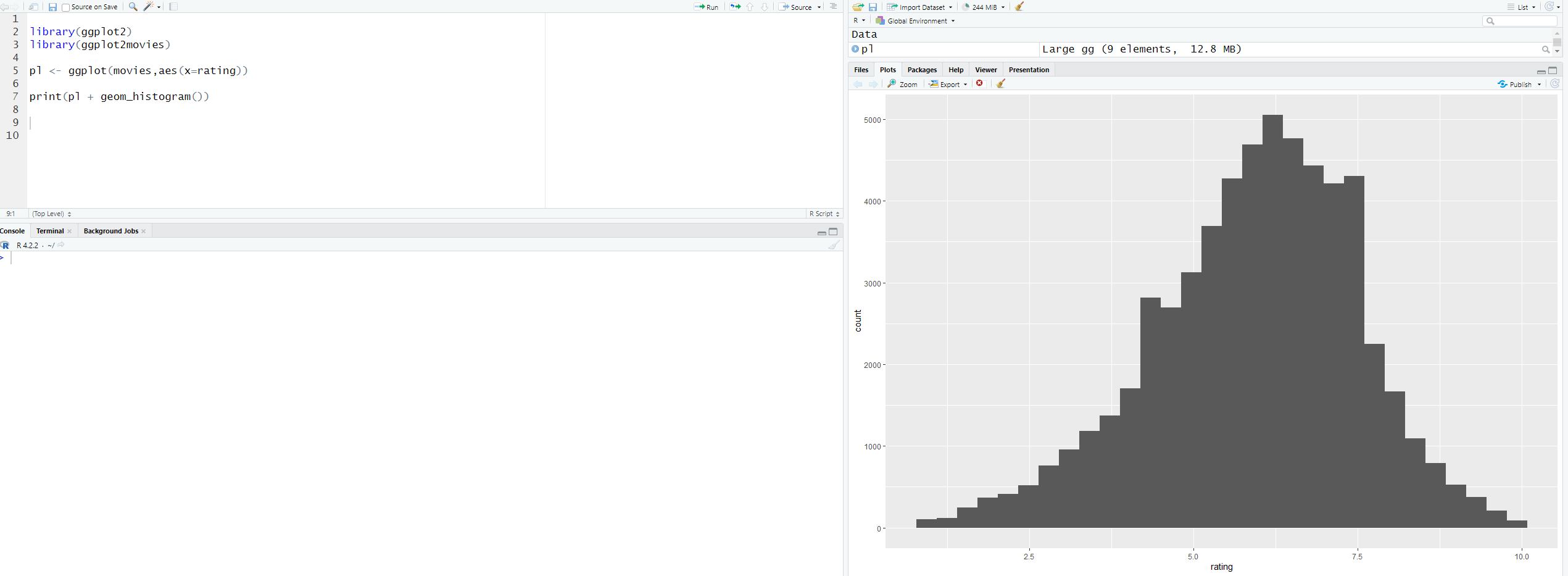
This is the basics of a histogram. We get the data from movies then we change the x-axis to rating and then we add geom_histogram() to create the histogram. The geom_histogram() is found in the cheat sheet, so reference your cheat sheet when creating types of graphs.

Bindwidth is changing how wide your bins are.
Color is changing the color.
Fill is filling in the bins (in the example blue is the outline while pink fills inside the bins)
Alpha is how transparent you want the bins

In this example, we use xlab and ylab to change the names of the x-axis and y-axis. I have also added a ggtitle to add the title to the histogram.
If you finished creating the histogram, you can export it into an image or pdf. You can also copy it to the clipboard. The export is located under plots on the right side.
Scatterplots

In this case, I have created a scatterplot using geom_point(). x is equal to wt, and y is equal to mpg. wt and mpg have to be the name from the dataset, you can’t just name it whatever you want.

You can change the color and transparency by adding what you want inside the parenthesis of geom_point().
size would change the size of the dots.
alpha is how transparent you want the dots to be.

This is a little bit more advanced. We have added a aes() inside the geom_point(). This would allow you to define sizes and shapes by other features or columns. In this case, by using size, the dots grow bigger as the horsepower grows bigger.
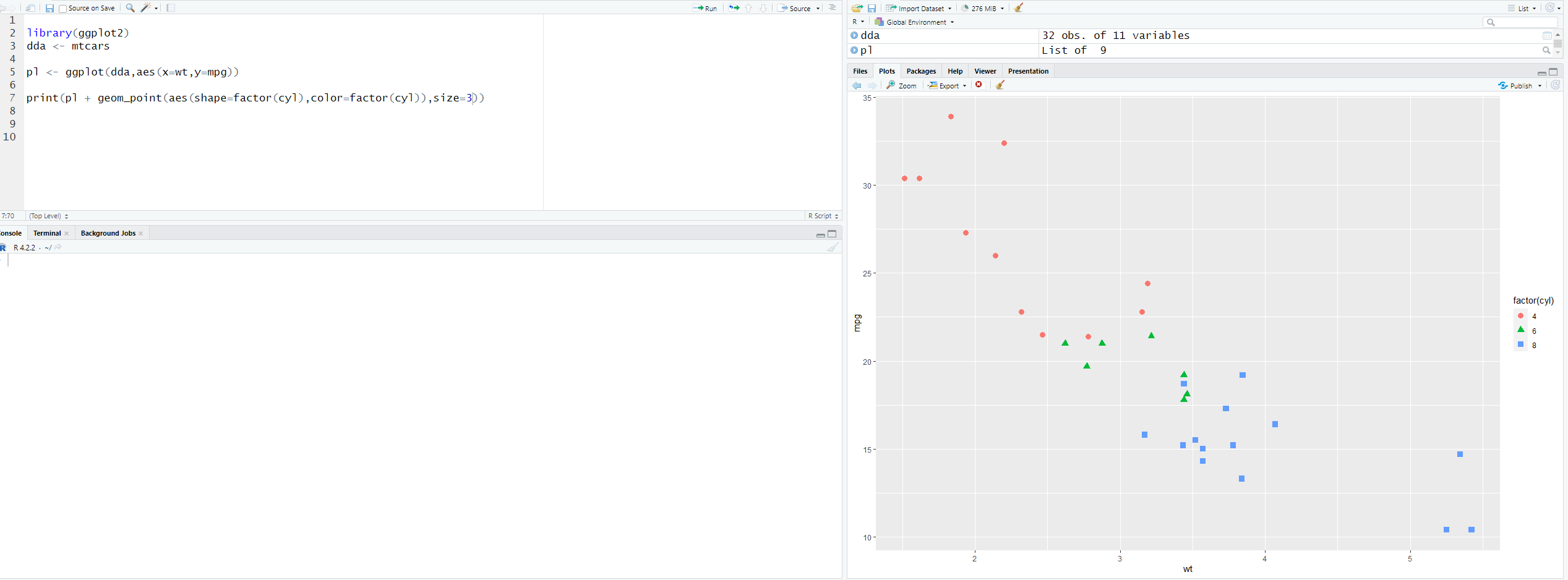
If you want to change the shape of the dots use shape=factor(‘data name’).
If you want to change the color of the dots use color=factor(‘data name’). You can put color outside aes(), but all dot colors would be the same, so if you want a different color for each shape, put color inside aes(). You can put a hex color, but the color has to be outside the aes().
Note that if you do this, the size has to be a whole number. You can’t put size=cyl (in my case) otherwise it would print an error. It must be a whole number like 1,2,3,4,5.
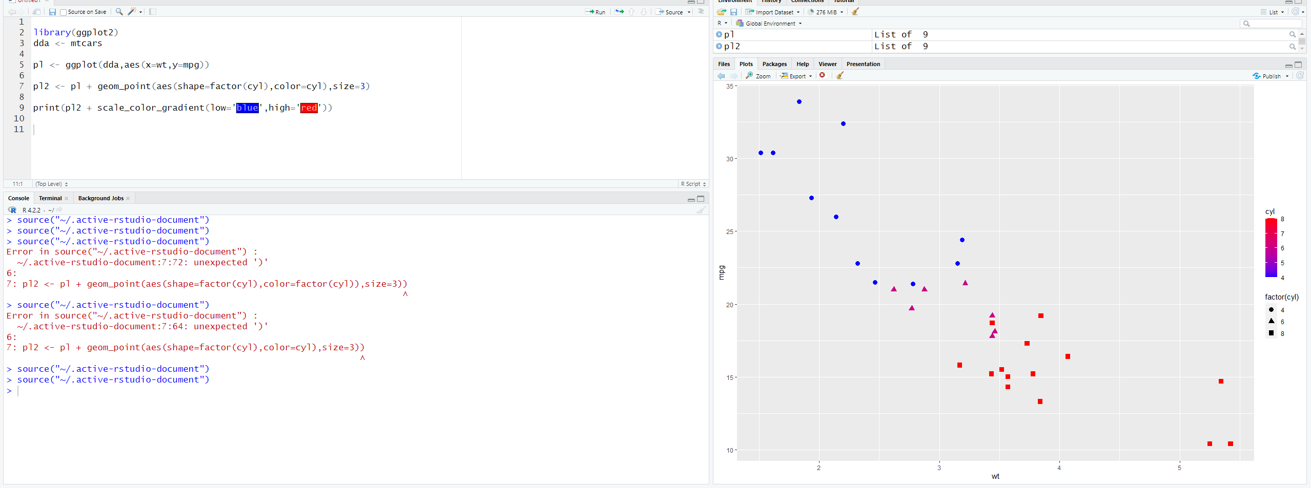
If you want to change color, you must change color=factor(‘data name’) to color=’data name’. You must also include scale_color_gradient(), a low color, and a high color.
Barplots

In this case, I have created a barplot using geom_bar(). x is the dataset name.
Like the histogram, we can also put color, fill, and alpha into geom_bar(). I’m not going to show that. Just reference the histogram and just change geom_histogram() to geom_bar().
[End of Part Six]
Part seven: Introduction to R for Data Science (Part Seven Final)