
The Beginner's Guide to Math with Python for Data Science (Part Two)
I thought I could win the lottery since other people have won it, but it turns out I was experiencing survival bias.

Inferential and Descriptive Statistics
Descriptive statistics are used to summarize data. Tools such as median, charts, mode, and bell curves are part of descriptive statistics.
Inferential statistics is the analysis process and will try to uncover attributes about a population.
Samples, Bias, Population
A sample is a subset of the population that is random and unbiased. We often have to use a sample because polling an entire population isn’t possible. Some populations might be easy to get and analyze, but that’s not always the case.
A population is a particular group we want to study. For example, we can study “all college students in the USA,” and “all high school juniors in Thomas Jefferson High School for Science and Technology.” We can have boundaries that define our population. It can be broad or can be specific. It just depends on what you want to analyze and study.
We would want our sample to be random as possible. If it isn’t random, then it may introduce some bias, meaning it skews our findings by overrepresenting a certain group. For example, if you want to analyze the median household income people make in the United States, then you want to gather data from everywhere. Now if you have just gone to one city and gathered all your data there, then it’s going to be skewed. One specific location can’t represent all.
Bias isn’t always geographic, there are many other factors that can influence our study. Here is a list of biases:
Confirmation bias - gathering data that supports your belief. For example, only following politicians that you agree with, which reinforces your beliefs.
Self-selection bias - when individuals are more likely to select themselves in the experiment.
Survival bias - focusing on survived/living subjects while decreased ones never take into account.

Just remember that computers and math don’t recognize bias in your data. Always ask how data is obtained, and then find out if that process has any biased.
Weighted Mean and Mean
Mean is the average of a set of values. Just add all the values and divide by the number of values.
Mean in Python:
sample = [2, 5, 8, 2, 9, 7, 4, 3]

mean = sum(sample) / len(sample)

print(mean)
There are two versions of mean: sample mean and population mean:

The summation symbol Σ means to add all the items together. The n and N represent the sample and population size.
If we want some values to contribute more to the mean than others, we would use weighted mean:

A common example is weighing exams and final exams. Let’s say we have two exams and a final exam. The two exams are worth 30% and the final exam is 40%. You’ve got an 83 on one exam and a 69 on another exam. For the final exam, you have gotten a 94 on it. We can use Python to calculate this:
sample = [83, 69, 94]
weights = [.30, .30, .40]

weighted_mean = sum(s * w for s,w in zip(sample, weights)) / sum(weights)

print(weighted_mean)
Median
The median is the middlemost value in a set of ordered values. You will order the values, and the median is the center value. In this example, 8 is the median as it’s the most center:
The median in Python:
sample = [0, 2, 5, 8, 9, 14, 18]

def median(values):
    ordered = sorted(values)
    print(ordered)
    n = len(ordered)
    med = int(n / 2) - 1 if n % 2 == 0 else int(n/2)

    if n % 2 == 0:
        return (ordered[med] + ordered[med+1]) / 2
    else:
        return ordered[med]


print(median(sample))
The median is useful when data is skewed by values that are extremely small or large than the rest of the values. It’s less sensitive to outliers.
Mode
The mode is the most frequently happening set of values. It’s useful for finding which values occur the most frequently. When no value happens more than once, there is no mode. When two values occur with equal amounts, then the dataset is considered bimodal.
The mode in Python:
from collections import defaultdict

sample = [2, 5, 3, 2, 7, 4, 8, 9, 2, 4, 2]

def mode(values):
    counts = defaultdict(lambda: 0)

    for s in values:
        counts[s] += 1

    max_count = max(counts.values())
    modes = [v for v in set(values) if counts[v] == max_count]
    return modes

print(mode(sample))Variance and Standard Deviation
Sometimes we want to find out how “spread out” the data is. You can find out how spread out the data is by finding the mean of all numbers and then subtracting the mean from each value. This will show you how far each value is from the mean.
This is the variance formula for the population:

Variance in Python (random numbers I’ve come up with):
data = [2, 4, 6, 9, 11, 23, 24]

def variance(values):
    mean = sum(values) / len(values)
    _variance = sum((v - mean) ** 2 for v in values) / len(values)
    return _variance

print(variance(data))
So the variance is 67.3469.
We would then have to find the standard deviation. This is the formula:

Standard deviation in Python:
from math import sqrt

data = [2, 4, 6, 9, 11, 23, 24]

def variance(values):
    mean = sum(values) / len(values)
    _variance = sum((v - mean) ** 2 for v in values) / len(values)
    return _variance

def std_dev(values):
    return sqrt(variance(values))


print(std_dev(data))
This would give us 8.20.
We do need to tweak the formula a little bit if we’re trying to calculate sample:


We do this to decrease bias in the sample.
So now if we’re trying to calculate standard deviation and variance in Python for a sample:
from math import sqrt

data = [2, 4, 6, 9, 11, 23, 24]

def variance(values, i_sample: bool = False):
    mean = sum(values) / len(values)
    _variance = sum((v - mean) ** 2 for v in values) / (len(values) - (1 if i_sample else 0))
    return _variance

def std_dev(values, i_sample: bool = False):
    return sqrt(variance(values, i_sample))


print(variance(data, i_sample=True))
print(std_dev(data, i_sample=True))
This would give me a variance of 78.57 and a standard deviation of 8.86. So if we were to recall our population variance/standard deviation, this sample version is much higher.
Z-scores
To turn x values into z score we have to use this formula:

Let me give you an example. Let’s say you live in neighborhood A and your friend lives in neighborhood B. Your neighborhood has a mean of $300,000 and a standard deviation of 5,000. Your friend’s neighborhood has a mean of 900,000 and a standard deviation of 15,000.
Now let’s say that your home is worth 320,000 and your friend’s home is worth 950,000.
So now if you want to find out which home is more expensive relative to the average home, then you would have to use the z formula:
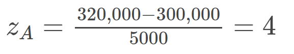

So this tells us that your neighborhood A is actually more expensive relative to its neighborhood than your friend’s neighborhood B since you have a z-score of 4 while your friend has a score of 3.33333.
Z-score in Python:
mean = 300000
std_dev = 5000
x = 320000


def z_score(x, mean, std):
    return (x - mean) / std

z = z_score(x, mean, std_dev)

print(z)
Vectors
I’ve written an article on Vectors.
Link: A Beginner's Guide to Understanding Vectors for Linear Algebra
But I’m going to give you a quick summary and how to write vectors in Python
In short, a vector is an arrow with a specific direction and length, which often represents a piece of data. It looks like this
In a graph:

2 is the x-axis while 5 is the y-axis.
To write vectors in Python:
v = [2, 5]
print(v)
You don’t really want to use plain Python for vectors, we should use the Numpy library instead since it’s more efficient.
To write vectors in Python using NumPy
import numpy as np
v = np.array([2, 5])
print(v)
We can also create three-dimensional vectors:
To write this in Python:
import numpy as np
v = np.array([2, 7, 9])
print(v)
We can just keep declaring more dimensions.
Adding vectors
We can add vectors together which is known as vector addition.
To add vectors together in Python:
from numpy import array

v = array([5, 8])
a = array([2, -3])

addition = v + a

print(addition)
Scaling Vectors
We can grow or shrink a vector’s length which is called scaling. It looks like this
Scaling in Python:
from numpy import array

v = array([2, 5])

scaling = 3 * v

print(scaling)
Scaling doesn’t change the direction, it only changes the magnitude. The only exception is multiplying a vector by a negative number which would flip the vector. Technically it doesn’t change the direction, it just flips it, but some people might think it changed direction.
[End of Part Two]
Great write up! Confirmation bias is extremely dangerous for decision making. Highly recommend reading the book “thinking fast and slow”. It goes into debt about decision making biases.
Keep up the great work!👍