
What is Bayesian Statistics? The Beginner Math Guide (Part Three)
Normal distribution... probably the most used meme in statistics

Normal Distribution
We’ll use the normal distribution to determine an exact probability for the degree of certainty that one estimate is more true than the other.
It uses the known mean and standard deviation as its two parameters.
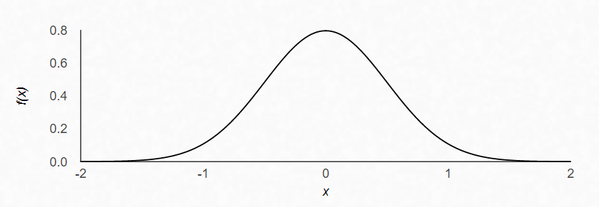
A normal distribution with a mean of 0 and standard deviation of 1 is shown as:

The center of the normal distribution is its mean. The width of the normal distribution is determined by standard deviation.
A normal distribution with a mean of 0 and standard deviation of 0.5 is shown as:
A normal distribution with a mean of 0 and standard deviation of 2 is shown as:

As standard deviation shrinks, so does the width of the normal distribution.
The normal distribution reflects how strongly we believe in our mean. So the more observations that are scattered, the less we are confident in the central mean.

Parameter Estimation
Say that you have a newsletter and you want to know the probability that a visitor will subscribe to your email list. In marketing, getting a user to perform a desired event is called a conversion event, or conversion, and the probability that a visitor subscribes to your newsletter is called the conversion rate.
Probability Density Function
The first tool we will use is the probability density function.
Let’s say that you have gotten 35,000 visitors and those visitors resulted in you gaining 200 subscribers.
So α = 200 and β = 34,800 (35,000 - 200 = 34,800):

We’ll also calculate the beta distribution mean:

Just divide the number of outcomes that we care about (200) by the total number of outcomes (35,000), so like 200/35000.
Ok, so we know that the newsletter's average conversion rate is:
200/35000 = 0.0057
or the mean of our distribution.
Because we have uncertainty in our measurement, it can be useful to find out how much more likely it is that the true conversion rate is 0.001 higher or lower than the mean of 0.0057 we observed.
To do this we’ll calculate 0.0047 and 0.0067

We’re trying to find out the true conversion rate between 0 and 0.0047.

Use R to do the calculation by the way:

In this one, we are trying to integrate 0.0067 to the largest value which is 1, to determine if the probability of our true values lies somewhere in this range.
We can visualize the PDFs using dbeta() in R:
xx <- seq(0.001,0.01,by=0.00001)
plot(xx,dbeta(xx,200,35000-200),type='l',lwd=3,
     ylab='Density',
     xlab='Probability of Subscription',
     main="PDF Beta(200,34800)"
)
Which results in:

We can also visualize the cumulative distribution function in R by:
xx <- seq(0.001,0.01,by=0.00001)
plot(xx,pbeta(xx,200,35000-200),type='l',lwd=3,
     ylab='Cumulative Probability',
     xlab='Subscription Rate',
     main="Cumulatve distribution function"
)
Which results in:
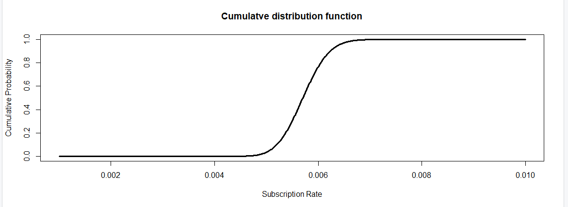
We can find the median, just by looking at this graph above, which is half of the value on one side and half on the other. It’s just the middle value of the data. The median is somewhere between 0.005 and 0.006. This is close to the mean of 0.0057.
Quantiles in R
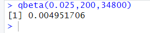
If we want to know the value that 99.9 percent of the distribution is less than, we can use qbeta():

The result is 0.0070, meaning that we can be 99.9 percent certain that our conversion rate is less than 0.0070.
To find a 95 percent confidence interval, we have to use a 2.5 percent lower quantile and values lower than a 97.5 percent upper quantile. This would give us a 95 percent confidence interval.
So for the lower bound:
For the upper bound:

Now we can say that we are 95 percent certain that our real conversion rate for newsletter visitors is somewhere between 0.49 percent and .65 percent.
We can use this to pin down estimate values for future events. For example, if one of your articles gets 100,000 views then based on our calculation, you should expect between 500 and 650 new email subscribers (100000 * .00653 = 650 (rounded)).
Bayesian A/B Test

Companies use A/B tests to try out emails, web pages, and other marketing materials to find out which one works the best for customers.
Say that you want to try out whether adding a meme image will help or hurt your conversion rate for your newsletter. For our test, we’re going to send one post with an image and another without. This is why it’s called A/B testing because we’re comparing variant A (with image) and variant B (without) to determine which one performs better.
Let’s just say that you have 400 subscribers. We’re only going to run the test on 200 of them.
The 200 subs will split into two groups, A and B. A will receive the image while B will have no image. So each group would have 100 subscribers
So we have sent out our emails and we have gotten these results:
                              Click                     Not click                      Observed Conversion rate

Variant A              29                                71                                         0.29

Variant B              67                                33                                          0.67
We do need a likelihood distribution, so I’m just going to use Beta(2,8) as my distribution.
We have to use beta distribution, making α the number of times it’s clicked and β the number of times it isn’t.
Recall:
So variant A will be represented by Beta(29+2, 71+8) and variant B by Beta(67+2, 33+8)
It’s pretty obvious that variant B has a higher conversion rate than variant B (from the data above), but the true conversion rate is a range of possible values, so to be sure that variant B has a higher conversion rate, we would have to use random sampling. The technique is known as Monte Carlo simulation.
So I’m going to use R to perform this sampling
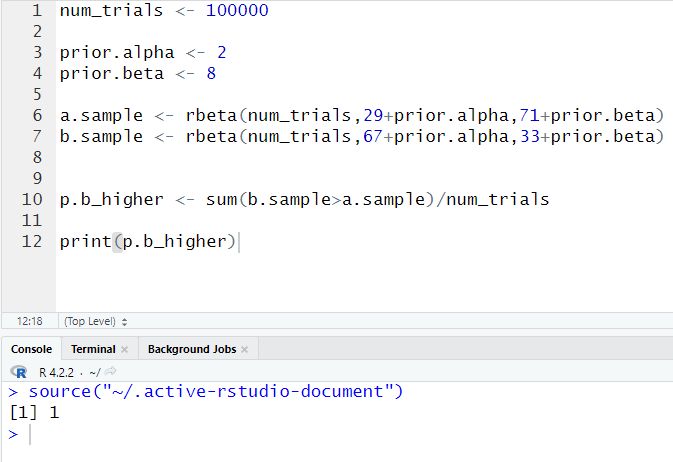
First, we started with 100,000 trials and we assigned them to num_trials.
Next, we put our prior alpha and beta values into variables.
Then, we collect samples from each variant. We use rbeta() for this.
Finally, we compared how many times that b.sample are greater than a.sample and divided that by num_trials, which would give us the percentage of the total trials where variant B is greater than variant A.
So the result we end up with was 1. So it means that 100 percent of the 10,000 trials, variant B was better.
[End of Part Three]