
What is Bayesian Statistics? The Beginner Math Guide (Part Two)
Don't you ever just love Bayes' theorem. The probability of this post going viral is one in a million. Well that's my guess at least.

Beta Distribution
You would use the beta distribution to estimate the probability of an outcome. Oftentimes, we’re given the probabilities for events, but in real life, that is rarely the case. We are given data instead which we have to use to come up with estimates for probabilities.
Data
I’m going to give you an example and some data.
Let’s say there is a gumball machine that will give you two gumballs if you put in a single quarter. However, there is a chance that the gumball will eat your quarter and will give you nothing in return. So you decided to test your luck.
You put in 1 quarter and the gumball machine gives you nothing. So you put in another quarter and all of a sudden the gumball machine gives you two gumballs. So you might guess that the probability at first is P(two quarters) = 1/2.
To have more data, you decided to use all your quarters and in the end, you get:
16 wins
29 losses
45 tries in total
So we have got two possible probabilities:
P(two quarters) = 1/2
P(two quarters) = 16/45
To make it easier, I’m going to assign a hypothesis:
We would want to calculate the binomial distribution to find out if 1/2 is useful for our data, so we would get the following:
So if H_1 was true and the probability of getting two gumballs was 1/2, then the probability of 16 occasions where we get two gumballs out of 45 trials would be .018.
If H_2 was true ad the probability of getting two gumballs was 16/45, then the probability of observing the same outcomes is .123.
So we have found out that H_2 is almost 10 times more probable than H_1.
Using Beta Distributions
Beta distribution will allow us to represent an infinite number of possible hypotheses. The probability density function is defined for continuous values. Here is the formula for the probability density function of beta distribution:

p represents the probability of the outcome
α represents how many times we have observed an outcome, such as getting two gumballs
β represents how many times the outcome we care about didn’t happen, so this is the number of times the gumball machine ate the quarter
Conditional Probability
Conditional probability depends on the outcome of a previous event.
Here is an example,
Let’s say that the probability of getting struck by lightning is 1 in 15,300. We can represent the probability as:
But let’s say that you are on a hilltop therefore the probability of you getting struck by lightning increased to 3/15,300 since lightning tends to hit high points. Now the probability of getting struck by lightning directly depends on whether you are on a hilltop since you have a higher chance of getting struck by lightning if you’re on top of a hill, thus this is an example of conditional probability. We can express it as P(A | B), or the probability of A given B. So this would look like:
We can read this as “The probability of getting struck by lightning, given that you are on top of a hill, is 3 in 15,300.”
We can look at the ratio of these two probabilities like,
Other factors can increase the probability of getting struck by lightning. For example, walking on an open field during a thunderstorm or standing in a boat on a lake can increase your chance of getting struck or standing in a boat on a lake. We can add all of this information, using conditional probability, to better estimate the chance of getting struck by lightning.

Bayes Theorem

The formula for Bayes’ theorem:
=\frac {P(B\mid A) \cdot P(A)}{P(B)}")
We can reverse conditional probabilities so that when we know the probability of P(B | A), we can use it to work out P(A | B).
Here is an example of the formula in use,
Let’s say that the rate of suicide is 3 percent for the entire population (this is fake data that I’ve come up with). While the entire population is 3 percent, males have a rate of suicide of 5 percent while females have a rate of 1 percent. We’ll also assume that the male/female split is 50/50.
So we get (these were divided by 100 to get the decimals, so like 3/100 = .03, 5/100 = .05, 50/100 = .5, etc):
So if we were to use Bayes theorem to find out the number of people who are male and suicidal we’d get:
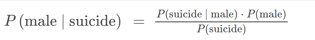
Which is:

Given the calculation, we know there is a 83.3 percent chance that males would commit suicide.
Bayes’ theorem will allow us to evaluate how much of our observed data changes our beliefs.

Spread of Data
Say that you and a friend wanted to drop some coins on top of a 3-story parking garage and time how long it takes for the coin to hit the ground. You tried it and you’ve got the following measurements in seconds:
4.02, 3.95, 3.98, 4.08, 3.97
But your friend wants to time it with other objects. So instead of coins, he uses a wide assortment of objects such as stones and twigs. Your friend would get the following measurements:
4.31, 3.16, 4.02, 4.71, 3.80
Both measurements have a mean of 4
Mean absolute deviation
We’ll measure the spread of each measurement from the mean. The mean for both measurements is 4. We’ll start by finding out the distance between the mean and the value:
Measurements                                                              Difference from mean (4)
     Group a
       4.02                                                                                         0.02
       3.95                                                                                        -0.05
       3.98                                                                                        -0.02
       4.08                                                                                         0.08
       3.97                                                                                        -0.03
     Group b
       4.31                                                                                         0.31
       3.16                                                                                        -0.84
       4.02                                                                                         0.02
       4.71                                                                                         0.71
       3.80                                                                                        -0.20
If we were to sum up their difference from the mean, both of them would equal 0:
The reason why we can’t sum up the difference is that the difference from the mean will cancel each other out.
We would have to take the absolute value of the difference. So that would mean that the absolute value of 5 is 5, and the absolute value of -5 is also 5. So | -5 | = | 5 | = 5.
So if we do this we’ll get:
We’ll then use the mean absolute deviation formula:
n is how many measurements you have got. So in group a I have gotten 5 different measurements.
In summary, it is just:
So for group a, the average observation is 0.04 from the mean.
For group b, the average observation is 0.416 from the mean.
This shows us that group b is about 10 times as spread out as group a.
Finding Variance
We could also find the variance since variance is easier to work with than taking the absolute value.
So the formula for variance is:
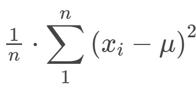
Which is just (this is group a):
Then we:
For group b:
Then we:
So for groups a and b, the variance is:
Var(group a) = 0.00212
Var(group b) = 0.269
In the case of variance, group b is now 100 times more spread out than group a.
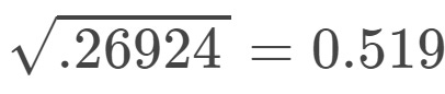
Standard deviation
It is hard to interpret the results for variance. So we’ll use standard deviation to fix it:

So in short, it’s (for group a):

For group b:
So in total for everything we get:
Method                                                               group a                                group b
Absolute deviations                                            0.040                                     0.416
Variance                                                               0.002                                     0.269
Standard deviation                                             0.046                                      0.519
[End of Part Two]