
Understanding the Different Types of Algorithms (Part Two)

Dijkstra’s Algorithm
You would use breadth-first search for finding paths with the fewest segments, but what if you want the fastest path instead? You can do so by using Dijkstra’s algorithm.
Let’s see how this works.

Each segment has a travel time in minutes. You’ll use Dijkstra’s algorithm to go from start to finish in the shortest possible time.
If you use a breadth-first search, it’ll take 7 minutes.
There are four steps to Dijkstra’s algorithm:
Find the node you can use to get the least amount of time
Update the costs of neighbors of this code
Repeat until you’ve done this for every node
Calculate final path
Step 1: It takes 6 minutes to get to node A, but only 2 minutes to get to node B. So node B is the closest node.
Step 2: Calculate how long it takes to get to all of node B’s neighbors by following an edge from B. If you go through node B, there is a path to A that only takes 5 minutes in total (2 + 3). So in this case, you found
A shorter path to node A
Step 3: Repeat
Step 1 again: So next we’ll repeat and find the least amount of time to get to the finish line. It’ll be 1.
Step 2 again: So now we found it takes 6 minutes to get to the finish line (2 + 3 + 1). At this point, you should know
It takes 2 minutes to get to node B
It takes 5 minutes to get to node A
It takes 6 minutes to get to the finish
The breadth-first search wouldn’t have found this as it isn’t the shortest path since it has three segments.
Terminology
When you work with Dijkstra’s algorithm, each edge in the graph has a number associated with it. This is called weights.
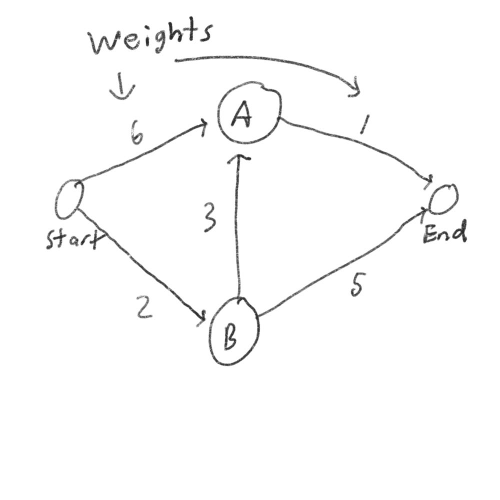
A graph with weights is called a weighted graph. A graph without weights is called an unweighted graph

To calculate the shortest path in an unweighted graph, use breadth-first search. To calculate the shortest path in a weighted graph, use Dijkstra’s algorithm. Also note: Dijkstra’s algorithm only works when all weights are positive. If weights are negative use the Bellman-Ford algorithm.
Graphs also have cycles. A cycle looks like this.

Greedy Algorithms
Suppose you have a classroom and you want to hold as many classes as possible. You made a list of all your classes, but you unnoticed that you can’t hold all of your classes here, because they overlap.
Now how do you pick what set of classes to hold, so that you can get the biggest set of classes possible?
Here is how you’ll do it:
Pick the class that ends the soonest. This is the first class you’ll hold
Now you’ll have to pick a class that starts after the first class. Again, pick the class that ends the sonnet. This is the second class you’ll hold.
Keep doing this, and you’ll end up with the answer.
A greedy algorithm is simple: at each step, pick the optimal move. In this case, each time you pick a class, you pick the class that ends the soonest. So in technical terms: at each step, you pick the locally optimal solution.
Sometimes greedy algorithms don’t always work.
The knapsack problem
Suppose you want to steal some goodies. You have a knapsack that can hold 35 pounds. You’re trying to maximize the value of items you put in your knapsack.
Using greedy algorithm:
Pick the most expensive thing that will fit in your knapsack
Pick the next most expensive thing that will fit in your knapsack. And so on
Except this wouldn’t work. Suppose there are three items you can steal.

Your knapsack can only hold 35 pounds. The VR headset is the most expensive, so you can steal that. Now you don’t have enough space for anything else. You got $3000 worth of goods.
But if you pick up the phone and laptop, you could have $3500 worth of goods.
So clearly greedy algorithm doesn’t give you the optimal solution. Greedy algorithm shines because they’re easy to write and usually get pretty close.
Dynamic programming
Let’s revisit the knapsack problem, but instead of 35 lbs, you can carry 30 lbs of goods.
You have three items you can put into the knapsack.

What items should you steal that will generate the most amount of money?
The simple solution
The simplest algorithm is this: you try every possible set of goods and find the set that gives the most value.
This works, but it’s slow. For three items, you have to calculate 8 possible sets. For four items, you have to calculate 16 sets. For every item you add, the number of sets you have to calculate doubles.
So how will we calculate the optimal solution?
This is how dynamic programming comes into play. Dynamic programming starts by solving subproblems and builds up to solving big problems.
For the knapsack problem, you’ll start by solving the problem for smaller knapsacks and then work up to solving the original problem.
Each dynamic-programming algorithm starts with a grid.

The grid starts out empty. You’re going to fill in each cell of the grid.
The laptop row
We’ll start with the first row. This is the laptop row, which means you’re trying to fit the laptop into the knapsack. At each cell, there is a decision: do you steal the laptop or not? Remember you’re trying to find the set of items that will give you the most value.
The first cell has a capacity of 10 lbs. The laptop is also 10 lbs, which means it can fit. So the value of this cell is $1500 and it contains the laptop.

Each cell will contain a list of items that will fit into the knapsack at that point.
Let’s look at the next cell. Here you have 20 lbs, well the laptop can fit there. The same goes for the next row, 30 lb.

This row represents the current best guess for this max. So right now the max you can get is $2000.
The phone row
The next one is for the phone. Now that you’re also in the second row, you can steal the laptop or the phone. Let’s start with the first cell, a knapsack with a capacity of 10 lb. The current max value you can fit into a knapsack of 10 lbs is $2000.
So should you steal the phone or not?
Well, the phone wouldn’t even fit inside the first cell as it’s 20 lbs. Because you can’t fit the phone, $2000 remains the max guess for a 10 lb knapsack.

On the 20 lb, the phone can fit, but the value is $1500 less than the $2000 laptop, so we would put a laptop for that place too.

Let’s skip the third cell for the phone row and move on to the VR headset, we’ll come back to that one when we finish the VR row.
For the VR row, it wouldn’t fit in the 10lb or 20lb cell, so we’ll put $2000 since that is our maximum. For the third cell, the value of the VR headset is $3000, so we can overwrite the $2000 laptop.
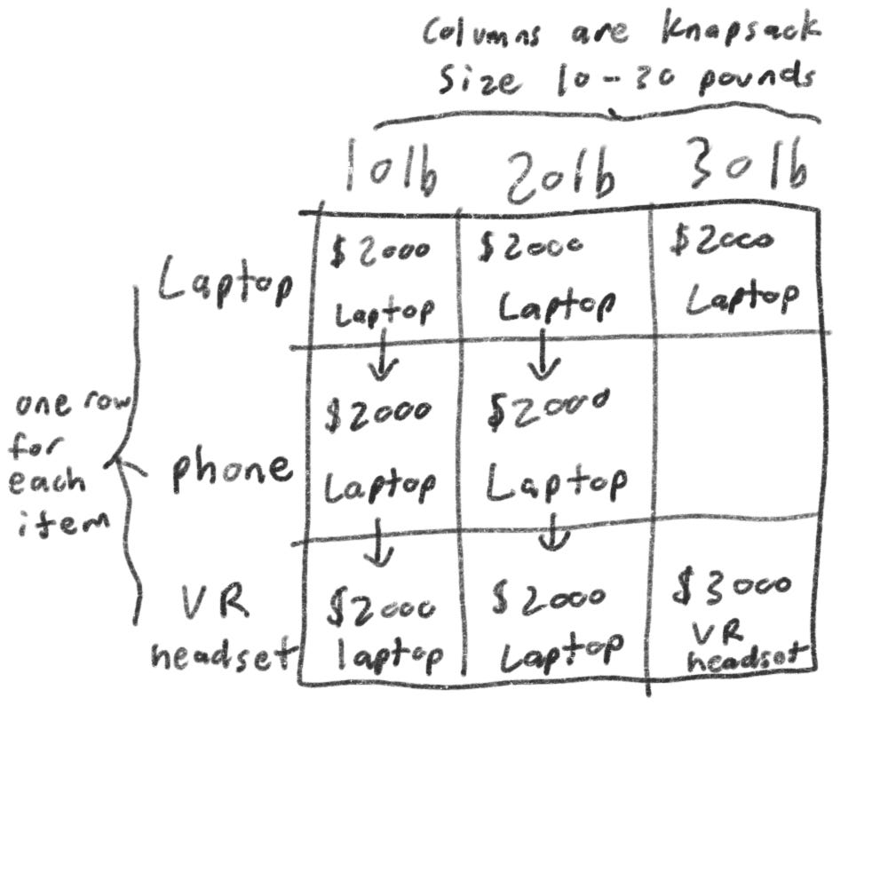
Back to the third cell for the phone row. We can notice the laptop only weighs 10 lb and the phone 20lb. Considering that we have 30 lb of space, we can fit two items there; the phone and the laptop. So now the maximum value is $3500 for that cell.
When you have space left over, you can use the answers to those subproblems to figure out what will fit in that space. It’s better to take the phone and laptop for $3500.

Suppose there is a fourth item you can steal. You don’t have to recalculate everything to account for the new item. Dynamic programming keeps progressively building on your estimate.
Sometimes the best solution doesn’t fill the knapsack completely. So if you have a diamond that is 25 lb and is worth $1 million dollars. You should steal it even if there is 5 lb left of space and nothing else can kit in that space.
Takeaways
Dynamic programming is useful when you’re trying to optimize something given a constraint. So in the knapsack example, you had to maximize the value of goods, constrained by the size of the knapsack.
You can use dynamic programming when the problem can be broken into discrete subproblems and they don’t depend on each other.
K-nearest neighbors
Let’s pretend you have a fruit. Is it an raspberry or a blueberry? Well, we know raspberries are bigger and redder than blueberries.
So the graph would look something like this
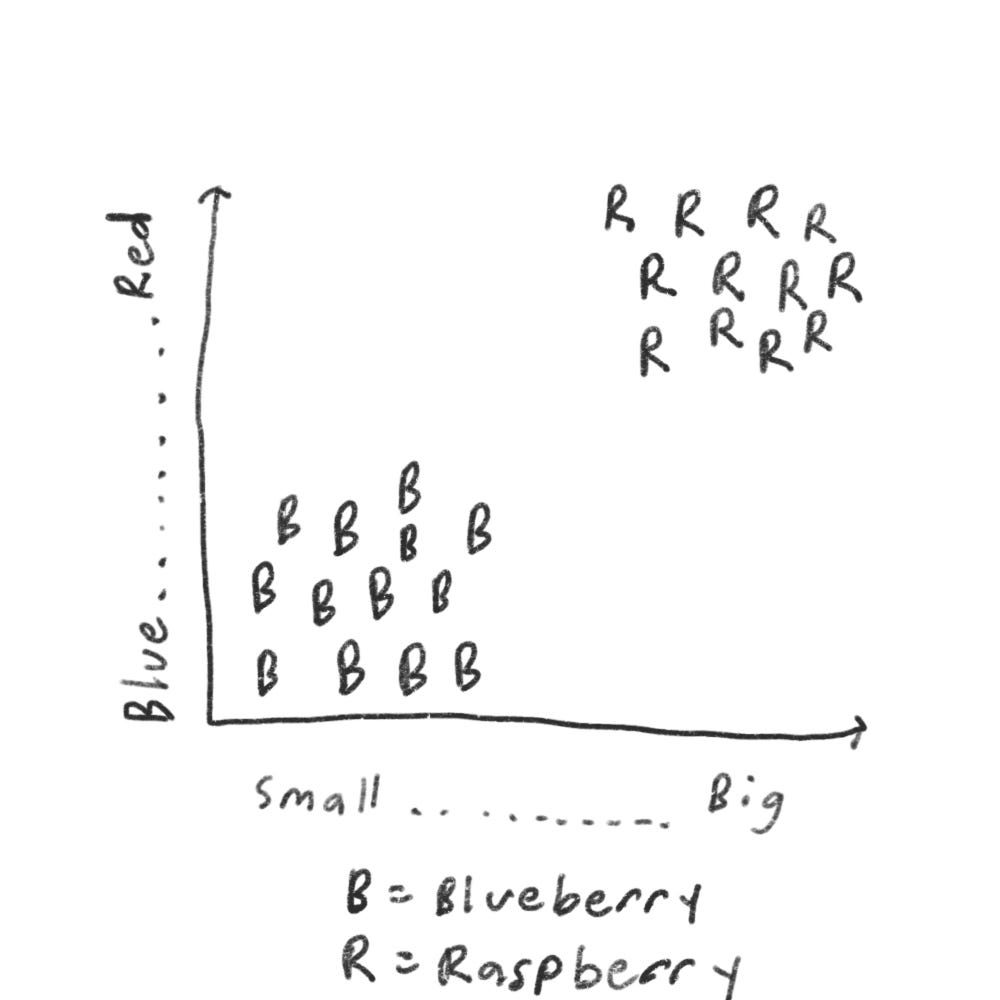
Generally, raspberries are bigger and red. So it’s easy to tell, but what if you get a fruit like this

How would you classify this fruit? One way is to look at the neighbors of this spot.
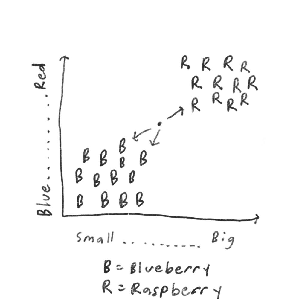
So more neighbors are blueberry than raspberry. So this fruit is probably a blueberry. This is k-nearest neighbors (KNN) algorithm.
The algorithm is simple:
You get a new fruit to classify
You look at its three nearest neighbors
More neighbors are blueberry, so this is probably a blueberry
We can graph by similarity. But how do you figure out how similar they are?
To find this, we would measure how close they are. To find the distance between two points, you use the Pythagorean formula.
We can use the distance formula to compare the distance between them, but another formula is to use cosine similarity. Suppose we have two users that are similar, but one of them is more conservative in their rating. They both loved Star Wars. David rated it 5 stars, but Josh rated it 4 stars. If you use the distance formula, these two users might not be each other’s neighbors even though they have similar tastes.
Cosine similarity doesn’t measure the distance, it compares the angles of the two vectors. It’s best at dealing with cases like this.
OCR
KNN is your introduction to machine learning. Machine learning is about making your computer more intelligent. OCR in particular stands for optical character recognition. It means you can take a photo of a page of text, and your computer will automatically read the text for you. How does it work?
Well, we can use KNN for this:
Go through lots of images of numbers, and extract features of those numbers
When you get a new image, extract the features of that image, and see what its nearest neighbors are
Spam filter
Spam filters use another algorithm called Naive Bayes classifier. First, you train your Naive Bayes classifier on some data.
Suppose you get an email with the subject “You’ve won 1 billion dollars collect now!” Is it spam? You can break this sentence into words. Then for each word, see what the probability is for that word to show up in a spam email. For example, in this model, the word billion only appears in spam emails. Naive Bayes figures out the probability that something is likely to be spam.
To Recap
KNN is used for classification and regression and involves looking at the nearest neighbors
Classification = categorization into a group
Regression = predicting a response
Feature extraction means converting an item into a list of numbers that can be compared
Picking good features is important
More algorithms
Here are some more algorithms I’m going to give a short brief about.
Trees
Let’s go back to the binary search example. When a user logs into Instagram, Instagram has to look through a big array if that username exists. But the problem is that every time a new user signs up, their username is inserted into the array. You’ll have to re-sort the array because binary search only works with sorted arrays. So wouldn’t it be nice if you could insert the username into the right slot in the array right away? That’s the idea behind the binary search tree.
A binary search tree looks like this
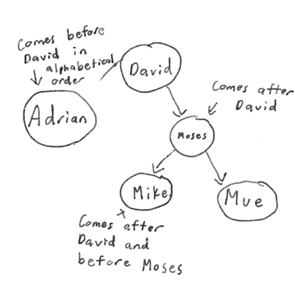
Suppose you’re searching for Mike. You start at the root node which is David.
Mike comes after David, so go toward the right.
Mike comes before Moses, so go to the left.
You would find Mike.
That’s basically the idea of binary search trees.
If you’re interested in more-advanced data structures or databases check out:
B-trees
Red-black trees
Splay trees
Heaps
Inverted indexes
This is a simplified version of how a search engine works. Suppose you have three web pages:
A = Hi
B = Hi There
C = We going
Let’s build a hash table from this content.
The keys of the hash table are the words, and the values tell you what pages each word appears on.

Suppose a user searches for Hi. We can see that it appears on pages A and B. Now suppose the user searches for There. We know it appears on pages A and C. This is a useful data structure: a hash that maps words to places where they appear. This is called inverted index and is commonly used to build search engines.
Ending
Here is a list of algorithms that I’m not going to touch upon, but may be useful to know:
Linear programming
Diffie–Hellman key exchange
Locality-sensitive hashing
Secure Hash Algorithms
Bloom filter
HyperLogLog
Distributed algorithms
Parallel algorithm
Fast Fourier transform
[End]