
Understanding the Different Types of Algorithms (Part One)

Binary Search
Suppose you’re trying to search for a person in a yearbook. Their last name starts with the letter J. Now you could start at the beginning and just keep flipping pages until you’ve reached J. But you’re most likely going to start in the middle because you know J will be near the middle of the book.
This is a search problem. It uses binary search to solve it.
Binary search is an algorithm used to find a specific element in a sorted list of elements. It works by repeatedly dividing the search space in half and comparing the target element with the middle component of the remaining portion. If the target element matches with the middle element then it returns it otherwise if the target element is smaller then the search continues in the lower half of the list while and if the target element is higher then it continues in the upper half. If it can’t find the target element it returns null.
Let’s take another example. Suppose you want to find a word in the Oxford English Dictionary. The dictionary has 600,000 words.
In a worst-case scenario, if you were to do a simple search it could take 600,000 steps if you’re trying to find a word that happens to be on the last page of the dictionary.
When it comes to binary search you would cut the number of words in half so it would look something like this:

In a worst-case scenario for binary search, it would take 20 steps (didn’t add decimal for some). This is a massive difference from the 600,000 steps it would take for a simple search.
Binary search does require the list to be sorted in order to work effectively. So something like a dictionary sorted in alphabetical order would work with binary search.
Time
You would want to choose the most efficient algorithm optimizing for either time or space.
When it comes to time you can save a lot when using binary search. If there is a list of numbers containing 100,000 words, it would take 100,000 steps for a simple search while a binary search would only take 16 steps. This is a massive saving in time.
Big O notation
Big O notation is a special kind of notation that will tell you how fast an algorithm is. For example, let’s say you have a size m list. A simple search will check each element, so it will take m operations. The run time for Big O is O(m). Big O doesn’t tell the speed in seconds. Big O would let you compare the number of operations. It’ll tell you how fast the algorithm grows.
Here are some Big O run times you’ll encounter, sorted from fastest to slowest:
O(log n), also known as log time. Example: Binary Search
O(n), also known as linear time. Example: Simple Search
O(n * log n). Example: fast sorting algorithm
O(n^2). Example: slow sorting algorithm, like selection sort
O(n!). Example: extremely slow algorithm
Here are some takeaways:
Algorithm speeds aren’t measured in seconds but in the growth of the number of operations
The run time of an algorithm increases as the size of the input increases
The run time of algorithms is expressed in Big O notation
O(log n) is faster than O(n), but it gets a lot faster as the list of items you’re searching grows
Selection Sort
How memory works
Imagine you want to store your two things. A chest of drawers is available. Each drawer can only hold one thing. You want to store two things, so you use two drawers.
That’s basically how computer memory works. Your computer looks like a giant set of drawers, and each drawer would contain an address.
Each time you want to store an item, you ask the computer for some space and it gives you an address where you can store your item. If you want to store multiple items, you can do so by using arrays and lists.
Arrays and linked lists
Sometimes you need to store a list of elements in memory. Should you use an array or a linked list? Using an array means all your tasks are stored contiguously (next to each other) in memory.
Let’s say you have four items. You can place three in the array, but one of them is taken up by some other thing. In cases like this, you can ask your computer for a different chunk of memory that can fit four tasks. Then you can move all your items there.
Linked lists
Items can be anywhere in memory with linked lists. Each item stores the address of the next item in the list. A bunch of random memory addresses are linked together.
Adding an item to a linked list is easy, you would just stick it anywhere in memory and store the address with the previous item. You never have to move your items. They are great if you’re going to read all the items one at a time: read one, follow the address to the next item, and so on. But if you’re jumping around, linked lists are bad.
Arrays are different. You know the address for every item in your array. You can look up any element in your array instantly. With a linked list, elements aren’t next to each other, so you can’t instantly calculate the position of the fifth element in memory.

The elements in an array are numbered. This starts from 0, not 1. The position of an element is called its index. For example, 4 is at index 1.
Selection sort
Suppose you have a bunch of songs on your computer and for each artist, you have a play count.

You want to sort this list from most to least played, so you can rank your favorite artist. How can you do it?
One way is to go through the list and find the most played artist. Add that artist to a new list. We’ll do it again to find the next-most-played artist. Keep doing this, and you’ll end up with a sorted list.

Selection sort is a cool algorithm, but it’s not very fast.
Recursion
Let’s say you want to open a locked suitcase. The key to the suitcase is in another box. That box contains more boxes, with more boxes inside those boxes. The key is in a box somewhere.
One approach to finding a key:
Make a pile of boxes to look through
Grab a box and look through it
If you find a box, add it to the pile to look through later
If you find a key, you’re finished
Repeat
Here is another approach:
Look through the box
If you find a box, go to step 1
If you find a key, you’re finished
The first approach uses a while loop. The second approach uses recursion. Recursion is where a function calls itself. Both approaches accomplish the same thing, but the second approach is more clear. Recursion is used when it makes the solution clearer. There is no performance benefit to using recursion, sometimes loops are better for performance.
Because recursive calls itself, it’s easy to write a function incorrectly that ends up in an infinite loop. When you write a recursive function, you have to tell it when to stop recursing. That is why every recursive function has two parts: the base case, and the recursive case. The recursive case is when the function calls itself. The base case is when the function doesn’t call itself again.
For example,
def count(i):
   print i
   if i <= 0:     (this is the base case)
      return
   else:          (this is a recursive case)
      count(i-1)
Stack
The call stack is an important concept in general programming and is also important to understand when using recursion.
Suppose you have a to-do list of all the things you want to do that day. You can add to-do items anywhere to the list or delete random items. When you insert items, it gets added to the top of the list. When you read an item, you only read the topmost item, and is taken off the list. So your todo list only has two actions: push (insert) and pop (remove and read).
This is called a data structure. The stack is a simple data structure.
Call stack
Your computer uses a stack internally called the call stack. Here is a simple function:
def greet(name):
    print("hello, " + name + "!")
    greet2(name)
    print("bye")
    bye()
This function greets you and then calls two other functions which are:
def greet2(name):
    print("How are you, " + name)


def bye():
    print("ok bye")
Suppose you call greet(“James”). First, your computer will allocate a box of memory for that call. The variable name is set to “James”. That needs to be saved in memory. Every time you make a function call, your computer saves the values for all variables for that call. Next, you print “hello, James! Then you call greet2(“James”).
Your computer is using a stack for these boxes. The second box is added on top of the first one. You print “How are you, James” and then you return from the function call. When this happens, the box on top of the stack gets popped off.
When you call the greet2 function, the greet function was partially completed. All values of the variable for that function are stored in memory.
Quicksort
Divide and Conquer
Suppose you have a plot of land. You want to divide this land evenly into square plots. You want the plots to be big as possible. Well, to figure out the largest square size you can use divide and conquer (D&C). D&C algorithms are recursive algorithms. To solve the problem using D&C, there are two steps:
Figure out the base case. This should be the simplest possible case
Divide or decrease your problem until it becomes the base case
First, figure out the base case. Suppose one side is 50 meters and the other side is 100 meters. Then the largest box you can use is 50 m x 50 m. You need two of those boxes to divide up the land.

Now you need to figure out the recursive case. According to D&C, with every recursive call, you have to reduce your problem. We can do so by marking out the biggest boxes you can use.

You can fit two 640 x 640 boxes in there, and there is still some left to be split up. Because there are some left to be split up, we can apply the same algorithm to this segment.
So before you started with a 1680 x 640 farm that needed to be split up. But now you need to split up the smaller segment, 640 x 400. If you find the biggest box that will work for this size, that will be the biggest box that will work for the entire farm. So we just reduced the problem from 1680 x 640 to 640 x 400 farm.
We can apply the same algorithm again starting with a 640 x 400m farm. The biggest box you can create is 400 x 400.
This would leave you with a smaller segment, 400 x 240 (640 - 400).
And then you can draw a box on that segment to get an even smaller segment, 240 x 160.
And then we can do it again and we’ll get 160 x 80.
If we split this one again too, we’ll be left with 80 x 80.
So the biggest plot size we can use is 80 x 80 m.
To recap:
Figure out a simple case as the base case
Figure out how to reduce your problem and get the base case
Quicksort
Quicksort is a sorting algorithm. It’s much faster than the selection sort.
Let’s use quicksort to sort an array. Some arrays don’t need to be sorted at all. Empty arrays and arrays with one element are some examples that don’t need to be sorted. You can return those arrays as is.
For a bigger array, one with two elements, it’s pretty easy to sort too.
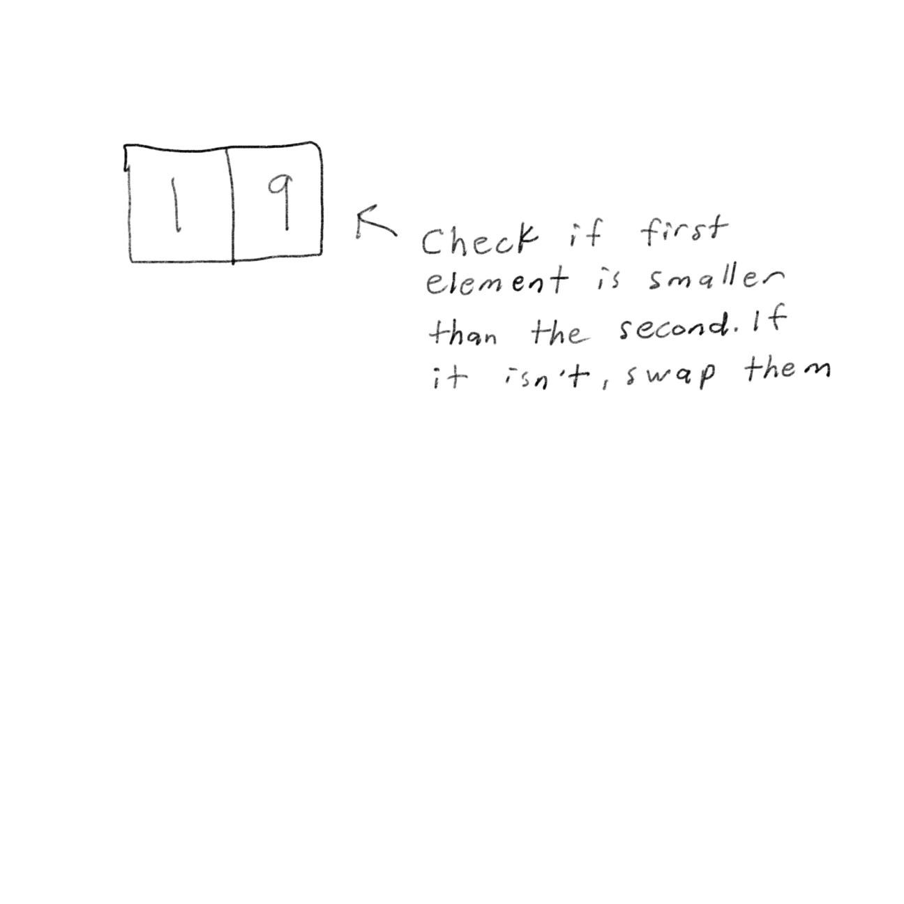
Now what about an array with three elements?
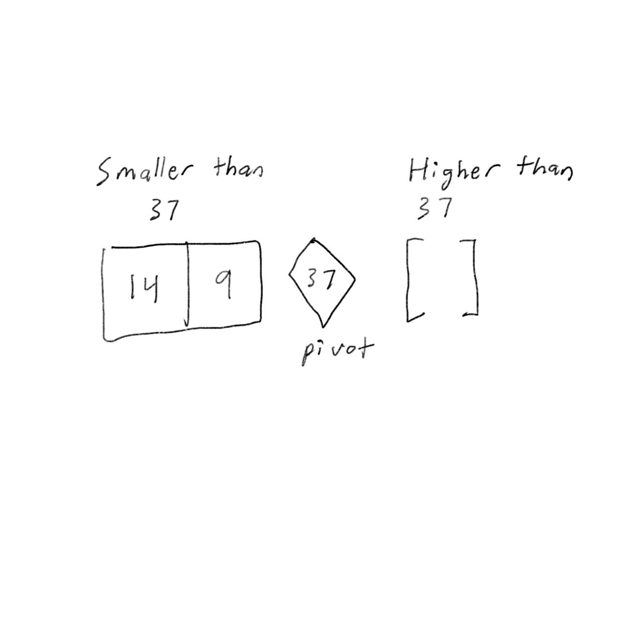
We can use D&C. We would want to break down the array until you’re at the base case. First, you’ll pick an element from the array. This element is called the pivot.

Now find the element smaller than the pivot and the elements larger than the pivot.
This is called partitioning. Now you have
A sub-array of numbers smaller than the pivot
Pivot
A sub-array of numbers greater than the pivot
The two sub-array isn’t sorted. If the sub-array is sorted, we can combine them like - left array + pivot + right array - which in this case would be [9, 14] + [37] + [] = [9, 14, 37], which is a sorted array.
Now what about an array with four elements?
Suppose you choose 37 again.
The array on the left has three elements. We can call quicksort on it recursively.
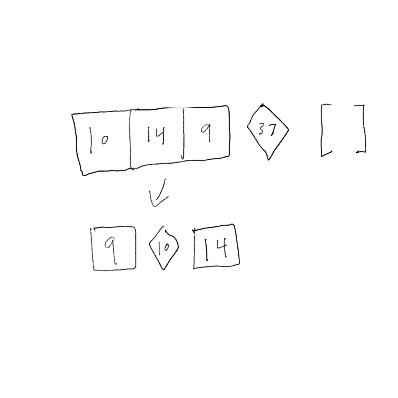
So now we can sort an array of four elements.
Here is the code for Quicksort:
def quicksort(array):
    if len(array) < 2:
        return array
    else:
        pivot = array[0]
        less = [i for i in array[1:] if i <= pivot]
        greater = [i for i in array[1:] if i > pivot]
    return quicksort(less) + [pivot] + quicksort(greater)


print(quicksort([2, 24, 3, 9]))
Quicksort speed depends on the pivot you choose.
Suppose you always choose the first element as its pivo and you call quicksort with an array that is already sorted. Quicksort doesn’t check to see whether the input array is already sorted. So it will try to sort it.
The best case is also the average case. If you choose a random element in the array as its pivot, quicksort will complete in O(n log n) time on average.
To recap:
If you’re using quicksort, choose a random lament as its pivot.
Hash tables
Suppose you want to look up the price of an orange in a book. The book is alphabetized, so it can take a long time for you to find the orange. You can use a simple search and binary search, but a better way is to find a person who has all the names and prices memorized. That way you don’t need to look up anything, you ask him, and he will tell you the answer instantly. He’ll be faster than binary search. This is where the hash function comes into play.
Hash functions
A hash function is a function where you put in a string and you’ll get back a number.
Here are some requirements for hash functions:
It needs to be consistent. Suppose you put in “orange” and get back “2”. Every time you put in “orange”, you should get “2” back. Without this, the hash table wouldn’t work.
It should map different words to different numbers. For example, it isn’t good if it always returns “3” for any word you put in. Every different word should map to a different number.
The hash function will tell you exactly where the price is stored. This works because:
Hash function consistently maps a name to the same index
Hash function maps different strings to different indexes
Hash function knows how big your array is and only returns valid indexes
Put a hash function and array together, and you’ll get a data structure called a hash table. Hash tables are also known as hash maps, dictionaries, maps, and associative arrays.
Python has hash tables called dictionaries. You can make a new hash table using dict:
item = dict()


item["apple"] = 0.70
item["orange"] = 0.89
item["candy"] = 1.50


print(item)
Let’s ask for the price of an orange:
print(item["orange"])This would print out 0.89.
In the item hash, the names of produce are the keys, and their prices are the values.
Cache
If you work with websites, you may have heard of caching. Here’s an example. Suppose you visit Instagram.com:
You make a request to Instagram’s server
The server thinks for a second and comes up with the web page to send to you
You get the web page
On Instagram, the server might be collecting all of your friends’ activity to show you. It takes a couple of seconds to collect all of it and present it to you. You might think why it’s so slow, but Instagram’s servers have to serve millions of people, and that couple of seconds add up for them.
This is how caching works: websites remember the data instead of recalculating it. If you logged into Instagram, all the content is tailored just for you. If you’re not logged in to Instagram, you see the login page. Everyone sees the same login page. Instagram is asked the same thing over and over: “Give me the home page when I’m logged out.” So it stops making servers do all the work to figure out what the home page looks like. Instead, it memorizes what the home page looks like and sends it to you.
Of course, Instagram isn’t just caching the home page. It’s also caching the About page, Help page, Jobs page, Terms page, and a lot more.
This is called caching and it has two advantages:
You get the web page a lot faster
Instagram has to do less work
Caching is a common way to make things faster. All big websites use caching.
Collisions
Suppose your array contains 8 slots and you assign a spot in the array alphabetically.
The problem is when you want to put the price of an apple in your hash it’ll be assigned in the first slot. This is a problem when another slot has been taken such as the price of a banana.

Now when you want to put the price of avocado in your hash. You’ll get assigned the first slot again.

Apples have already taken that slot already. This is called a collision: two keys have been assigned the same slot. If you store the price of avocados, it’ll overwrite the price of apples. The next time someone asks for the price of apples, they’ll get the price of avocados instead.
There are different ways to deal with collisions. The simplest one is to start a linked list at that slot.

In this example, avocados and apples are in the same slot, so you start a linked list at that slot. If you need to know the price of bananas, it’ll be quick, but if you need to know the price of apples then it’ll be a little slower. You’ll have to search through the linked list to find apples. If the linked list is small, then it’s not that big of an issue.
If linked lists do get long, it could slow down your hash table a lot.
You’ll almost never have to implement a hash table yourself. You can use Python’s hash tables and assume you’ll get the average case performance.
Breadth-first Search
Breadth-first search will allow you to find the shortest distance between two things.
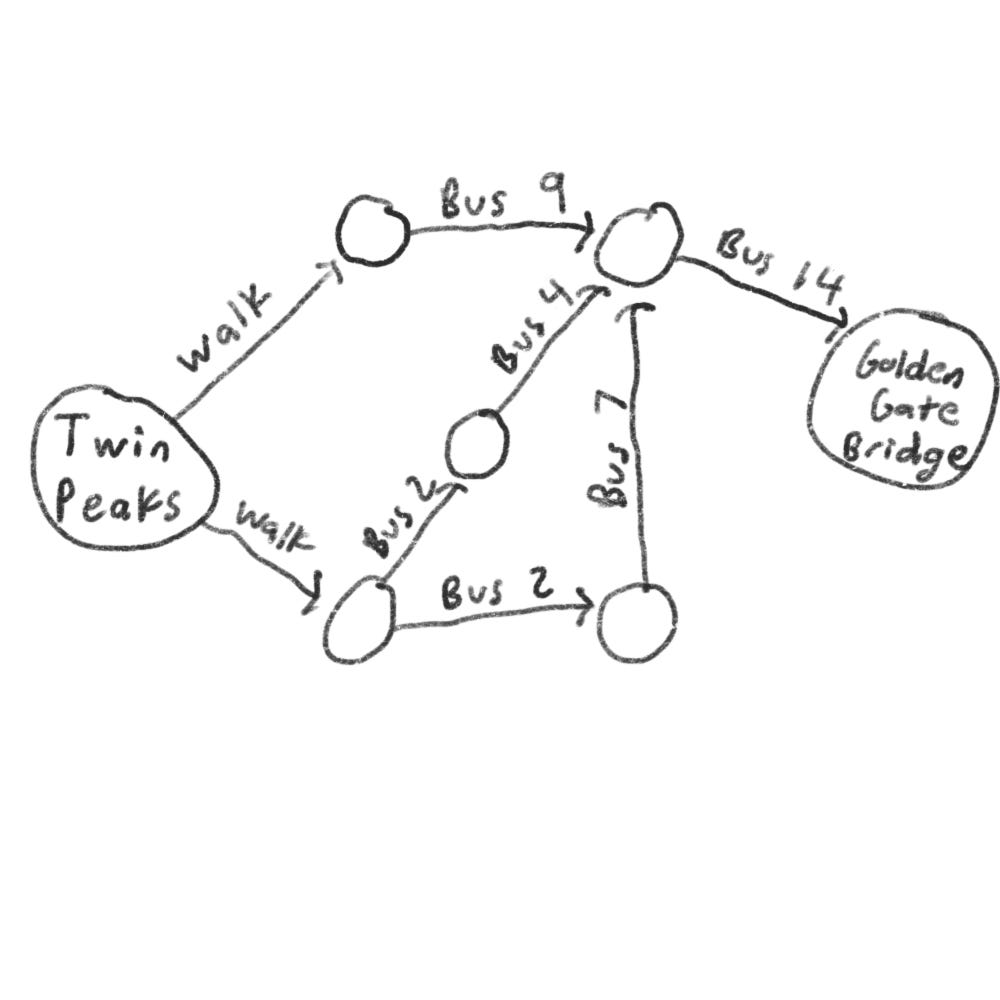
Suppose you’re in San Francisco and you want to go from Twin Peaks to the Golden Gate Bridge. You want to get there by bus with the least amount of transfers. Here are your options,
What’s the algorithm to find the path with the fewest steps?
Well, we can’t get there with just one step.
We also can’t get there by taking two steps.
But we can get there with three steps, so it would take three steps to get from Twin Peaks to the bridge using “walk” then “Bus 9” and then “Bus 14”.
There are other routes, but they are longer. The algorithm found the shortest route to be three steps long. This type of problem is called shortest-path problem. You’re always trying to find the shortest something. The algorithm to solve the shortest-path problem is called breadth-first search.
There are two steps:
Model the problem as a graph
Solve the problem using a breadth-first search
Graph
A graph models a set of connections. Each graph is made up of nodes and edges. A node can be directly connected to many other nodes. Those nodes are called neighbors.

Here is another example of a breadth-first search:
Suppose you want to find an apple seller who can sell your apples. To find them, you can search through your friends on Facebook.
First, we’ll make a list of friends to search.
Then go to each person on the list and check if that person sells apples
Suppose none of your friends are apple sellers. Now you have to search through your friends’ friends.
Each time you search for someone from the list, add all of their friends to the list.
This way you can search for your friend and also their friends too. So if James isn’t an apple seller, you add his friends to the list too. That means you search for his friends and then their friends, and so on. With this algorithm, you’ll search your entire network until you come across an apple seller. This algorithm is a breadth-first search.
Recap:
There are two questions breadth-first search can answer:
Is there a path from node A to node B?
What is the shortest path from node A to node B?
Queues
Suppose you and your friend are queueing up at a bus stop. If you’re before him in the queue, you can get on the bus first. Queues are similar to stacks. You can’t access random elements in the queue. Instead, there are two operations, enqueue and dequeue.
Enqueue would add an item to the queue.
Dequue would take off an item from the queue.
The queue is called a FIFO data structure: First In, First Out. A stack is called a LIFO data structure: Last In, First Out.
Implementing the algorithm
Here is how it’ll work,

Sometimes Bob and Josh might share a friend: David. So David will be added to the queue twice. You’ll end up with two Davids in the search queue, but you only need to check David once to see whether he’s an apple seller. If you check him twice, you’re doing extra work. So once you search for a person, mark that person as searched and not search for them again.
If you don’t do this, you could end up in an infinite loop, so just keep a list of people you’ve already checked.
[End of Part One]