
A Beginner's Introduction to Matrices for Linear Algebra
When you got to multiply each row by each column in a matrix 😢

Matrices
A matrix is a rectangular array of numbers written between rectangular brackets, such as
You can also write it in parentheses instead of rectangular brackets, such as
The size or dimensions of a matrix refers to the number of rows and columns it has. In this case, the matrix above has 3 rows and 4 columns, so the size is 3 x 4.
The elements of a matrix are the individual values that make up the matrix. For example, the element in the i-th row and j-th column of a matrix A is denoted by A(i,j). Positive integers of i and j are called indices.
Two matrices are considered equal if they have the same dimensions (same number of rows and columns) and their corresponding entries are equal.
Square matrix
A square matrix is a matrix that has an equal number of rows and columns. A square matrix of m x m is called order m. The same for n x n (order n).
There is tall matrix that has more rows than columns and also wide matrix that has more columns than rows.
Row and column vectors
A vector with n elements can be represented as an n x 1 matrix, and there is no distinction made between matrices with a single column and vectors. A matrix with only one row is called a row vector. Example,
A matrix with only one column is called a column vector. Example,
Matrix example
Well here is a specific example of a 2 x 3 matrix
The first row is,
which is a 3-row-vector or 1 x 3 matrix, and second column
which is a 2-vector or 2 x 1 matrix.
Block Matrices
Here is an example,
The matrices are b, c, d, and e. These are called block matrices; the elements b, c, d, and e are called blocks of a. You can refer to them by their row and column, for example, d is the 1,2 block of a.
Matrix blocks that are placed side-by-side in the same row are called concatenated. When matrix blocks are placed above then they’ll be called stacked. For example, let’s say that you have these matrices,
The block for a would then be,
Zero matrix
A zero matrix is a matrix where all its elements are zero. It is denoted by the symbol 0 or 0_m x n, where m x n represents the size of the matrix. When a matrix is multiplied by a zero matrix, the resulting matrix is always a zero matrix.
Identity matrix
Identity matrices are pretty common matrices. It’s a square matrix that has ones on its main diagonal (from the upper left to the lower right) and zeros everywhere else. It is denoted by I, and its size is indicated as a subscript. For example, I_2 is the identity matrix of size 2 x 2.

Diagonal matrices
A diagonal matrix is a square matrix where only non-zero elements are located on the diagonal that goes from the top left to the bottom right of the matrix. The off-diagonal elements of a diagonal matrix are all zero. Diagonal matrices are often denoted as diag(a_1, a_2, ..., a_n).
So if we have,
diag(-5, 0)
we’ll get,
If we have,
diag(2, 4, 1.9)
we’ll get,
Matrix Transpose
A matrix is denoted as A^T if it’s transposed. So if A is m x n, then A^T is n x m. Here is an example,

We can get back the original matrix if we transpose it twice: (A^T)^T = A. Basically it converts row vectors into column vectors, same goes vice versa.
The concepts that apply to column vectors can also be extended to row vectors by taking their transpose. If a collection of row vectors is linearly dependent, it means that the transposes of those row vectors ( which are column vectors) are also linearly dependent.
We can also transpose block matrices such as
Matrix addition
Two matrices can be added together if they’re the same size. For example,
Matrix subtraction is similar. For example,
Remember that I_2 is a 2 x 2 identity matrix.
Multiplication
Similar to how vectors are multiplied. For example,
Matrix norm
The equation is,

The norm of a matrix is a numerical value that reflects the size or magnitude of the matrix. The norm is nonnegative homogeneous. The concept of matrix norm enables us to quantify the difference between two matrices and define how close or far apart they are. If the distance is small, then they are similar, whereas if they’re large, they are dissimilar.
Matrix-vector multiplication
Here is a simple example,

This multiplication table shows a good idea of the logic behind it,

Geometric transformations
Geometric transformations such as rotation, scaling, and reflection of points in two-dimensional space can be expressed as matrix-vector products. Specifically, given a 2 x 2 matrix A and a two-dimensional vector x representing a point, the product Ax yields a new vector y that represents the transformed point.
Scaling
Scaling changes the length of a vector. When scalar a is positive, it stretches the vector by a factor of |a|, and when it is negative, it also flips the direction of the vector.
Dilation
Dilation stretches a vector x by different factors along different axes. This can be done using a diagonal matrix D. If D is the diagonal matrix with diagonal entries d1 and d2, then the transformation can be expressed as y = Dx, where y is the transformed vector.
Rotation
Matrices will rotate a vector counterclockwise by 0 radians. Such as,

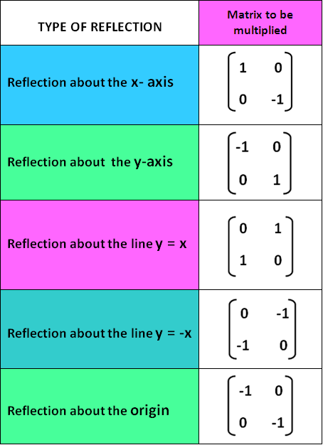
Reflection
Matrix will be reflected. This image sums it up,
Incidence matrix
A directed graph is a collection of vertices or nodes that are connected by edges. Each edge in the graph connects two nodes, one called the starting node, and the other called the ending node. The graph can be represented as a set of vertices and edges, where the vertices are labeled 1,...,n and the edges are labeled 1,...,m. The incidence matrix can be described as a directed graph by the n x m matrix.

Networks
A graph is often used to model a network, where the nodes represent entities and the edges represent connections between them. Edges in a network can represent many different types of relationships, such as communication pathways, or traffic flow. The direction of an edge may or may not indicate the direction of flow in the network, depending on the application. In many cases, we can define a set of rules to determine the direction of flow based on the direction of the edges.
Flow conservation
Flow conservation can be applied to a network represented by a graph. If we assign flow values to the edges, we can use linear equations to model the flow of the quantity through the network. If the total flow into a node equals the total flow out of the node, we say that flow conservation occurs. When the flow vector x satisfies Ax = 0, it is called a circulation, and it can be used to model traffic flow through a network of roads.
Sources
Sometimes it’s beneficial to include additional flows called source flows, that will enter or leave the network at the nodes, but not the edges.
Linear dynamical systems
A linear dynamical system describes how a system evolves over time, where the variation of a state vector is determined by multiplying the vector by a constant matrix. It is a simple model in which each x_m+1 is a linear function of x_m:

The n x n matrices, A is called the dynamics matrices. The equation above is called the dynamic equation. If we have the current value of x, we can predict all future values, without the need to know the past states.
We can add more terms to the equation:

The u_m is called the input (could also be called an exogenous variable), B_m is called the input matrix of n x m, and the c_t is called the offset.
Matrix multiplication
We can multiply two matrices together using matrix multiplication. You can only do so if the number of columns of A equals the number of rows of B.
Here is an example,

The math behind it,
1(1) + 3(3) + 2(0) = 10
1(2) + 3(-1) + 2(1) = 1
5(1) + -1(3) + 0(0) = 2
5(2) + -1(-1) + 0(1) = 11
If you want to know the formula for multiplying two 2 x 2 matrices,

Gram matrix
A Gram matrix is formed by taking the dot product of each pair of vectors in a set of vectors and placing the results in a matrix. It can be expressed as

The entries of G give all inner products of pairs of columns of v. Remember that the Gram matrix is symmetric, since v_i * v_j = v_j * v_i.
Orthonormal
As an application of Gram matrices, we can use them to check if a set of vectors v_1, ...,v_n are orthonormal. We can do so by:
where V is the k matrix with columns v_1,…,v_k. When a square matrix satisfies V^TV = I, where V is the square matrix, it is called an orthogonal matrix.
QR factorization
It is a decomposition of matrix A into,
This is called QR factorization of A since it expresses A as a product of two matrices, Q and R, where Q has orthonormal columns and R is upper triangular with positive diagonal elements. If A is square, then Q is orthogonal.
The equation Q^TQ = I follows the orthonormal of vectors q_1,…,q_k. The R is upper triangular since each vector a_i is a linear combination of q_1,…,q_i.
Matrix Inverse
A matrix B that satisfies
is called the left inverse of A.
A matrix B that satisfies
is called the right inverse of A.
If a matrix is both left- and right-invertible, then it is invertible and its inverse is unique. So let’s say that AB = I and XA = I (B is any right inverse and X is any left inverse), we’ll have,
where the left inverse of A would match the right inverse of A. When a matrix has a right inverse of B and a left inverse of X, we call it B = X and it’s an inverse of A, denoted as A^-1. The A would be called invertible. Invertible matrices must be square though.
QR factorization inverse
The Q and R are invertible, and the formula is
where R^-1 is the inverse of the upper triangular matrix R, and Q^T is the transpose of the orthogonal matrix Q. This will give us a simple option to compute for matrix inversion, especially the large matrices.
[End]