
The Beginner's Guide to Math with Python for Data Science (Part One)
The most basic math guide I could come up with.

Note:
Python will be used.
This is not a comprehensive review of math
Numbers
Here are some different number systems:
Natural numbers: Numbers such as 1, 2, 3, 4, 5, 6… so on. Only positive numbers here.
Whole numbers: Same as the natural number, but zero is now added, so it’s 0, 1, 2, 3, 4… so on.
Integers: They include both positive and negative natural numbers as well as zero.
Rational numbers: Numbers that you can express as a fraction such as 1/3, is a rational numbers. This includes finite decimals and integers since they can also be expressed as fractions. They are called rational since they are ratios.
Irrational numbers: These are numbers that can’t be expressed as fractions such as π, square roots, and Euler’s number.
Real numbers: They include both rational and irrational numbers.
Order of Operations
The order of operations is the order that you solve for each part of the equation. So for example,
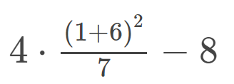
First, you would solve the parentheses (1 + 6), which equals 7:
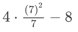
Then we will solve the exponent, which is squaring 7. That is 49:

Next is multiplication and division. We’ll multiply first which gives us 196 (4 * 49):

Now we divide 196 by 7, which gives us 28:
Now we subtract and it’ll give us 20:
We could take the easy way out and use Python:
answer = 4 * (1 + 6)**2 / 7 - 8

print(answer)
You can also put parentheses for clarity:
answer = 4 * ((1 + 6)**2 / 7) - 8

print(answer)
Both are correct, but one is just more clear. When coding always choose the option that is more clear to us humans.
Variables
A variable is a placeholder for an unknown number. You can have a variable representing a real number, and you can divide that number without declaring what it is. In this example, we have a variable a and divided it by 2:
a = int(input("Please give me whole number? \n"))

outcome = a / 2

print(outcome)
Functions
Functions define the relationship between two or more variables. Functions take input variables and then plug them into an expression, and the result is an output variable (or called a dependent variable).
For example,
For any value of x, we can plug it into 3x. When x = 1, then y = 12 since 3(1) = 3 + 9 = 12. When x = 2, y = 15, and so on.
You may see the dependent variable y label as the function of x, such as f(x). So rather than y = 3x + 9, it is expressed as:
We can declare a function in Python by:
def f(x):
    return 3 * x + 9

x_number = [0, 1, 2, 3, 4, 5]

for x in x_number:
    y = f(x)
    print(y)
This is a graph for function y = 3x+9. When we plot on a two-dimension plane with two number lines, it is called a x-y plane, or coordinate plane.
Summations
Summation is expressed as a sigma ∑ and adds elements together. So if we want to iterate the numbers one through five, multiply each by three, and sum them:
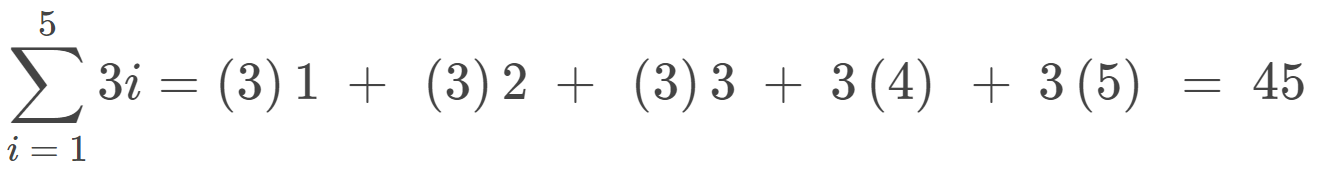
In Python, we can write this as:
output = sum(3*i for i in range(1,6))
print(output)
Exponents
Exponents are multiplying the number by itself a specified number of times. So when you have 2^4, it is multiplying four twos together:
Multiplying x^3 and x^5 together is different:
When we multiply exponents together, we add the exponents, which is known as the product rule.
For division:
When we divide x^3 by x^5 we cancel out three x’s leaving us with 1/x^2. 1/x^2 is the same as x^-2, so you can use whatever you want.
Any base with an exponent of 0 is 1. The reason is that when a number divides itself, it will equal 1, so you have x^0 / x^0 which equals 1. Same with x^2 / x^2 = 1,…etc.
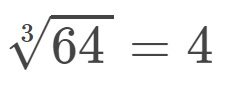
A cubed root is similar to square roots, but they want numbers multiplied by a specific value, so a cubed root of 64 is expressed as 3sqrt64. It basically means that the number multiplies itself by three times which will give us 64. This would be 4 as 4 * 4 * 4 = 64.
One last thing, an exponent of an exponent will multiply the exponents together, which is known as the power rule. So for example,
Logarithms
A logarithm is a math function that determines the power to which a given base must be raised to obtain a specific number. One way to think of this is by asking yourself “4 raised to what power gives me 256.” We can express this mathematically by using x for the exponent:
It’s pretty simple to know the answer is 4, but we need a way to express this. This is what the log() function is used for.
It’s basically:
We can use the log function in Python
from math import log

x = log(256, 4)

print(x)
Here are some properties:
")
Euler’s Number
Euler’s number e sometimes shows up. It’s a special number like Pi π and its numerical value is 2.71828183. We use e as a way to simplify things.
For example, let’s use the formula to calculate interest:
P is the starting investment
r is the interest rate
t is the number of years
n is the number of months in each year
So let’s calculate a 100 starting investment, 12% interest rate, 12 months, 2 years. This would compound monthly(12), so a 12% increase per month for 2 years
If we wanted to do this in Python:
p = 100
r = .12
t = 2
n = 12

a = p * (1 + (r/n))**(n*t)

print(a)
But let’s say that we want to compound daily, we’ll have to change n to 365:
Well, that is a small difference, let’s try compounding every minute (525600 minutes in a year):
Now we are getting smaller fractions the more frequently we compound. We can simplify things by using Euler’s number e, which is a formula to compound “continuously”, meaning nonstop:
So if we calculate our investment after two years:
Not too surprising since compounding every minute got us 127.1249.
We can use e in Python using exp() function:
from math import exp

p = 100
r = .12
t = 2

a = p * exp(r*t)

print(a)
Natural Logarithms
When we use e as a base for logarithm, it’s called natural logarithm. Depending on the situation, we can use ln() instead of log(). So for example:
However, in Python, a natural log is specified as log(). So calculating natural logarithms of 49 in Python:
from math import log

a = log(49)

print(a)
Limits
Let’s take the function:

When we are looking at positive x values, we can see that as it increases, f(x) gets closer to 0. The thing is, it never actually reaches 0, it just gets closer. So it’s basically infinity. This can be expressed through a limit:
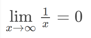
You can read this as “when x approaches infinity, 1/x approaches 0, but never reaches 0.”
Derivatives
Derivatives will help us measure the rate of change at any point in a function. So when we encounter an exponential function like f(x) = x^3, the derivative is 3x. So if we want to find the slope at x = 3, we can:


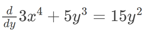
Partial Derivatives
These are derivatives that have multiple input variables. The x and y variable will get their own derivative. So if we want to find:
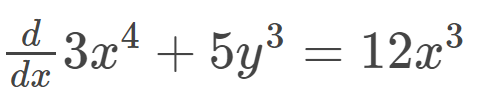
It’s 12x^3 since 3 * 4 = 12 and x^{4-1} = x^3.
Basically:

Chain Rule
Let’s start with an example,
These functions are linked because y is the output variable while the input variable is the second. This means we substitute the first function y into the second function z,
So our derivate would be:
We can also use a different approach:
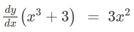


If we substitute y with x^3 + 3, it will equal 6x^2(x^3 + 3):
[End of Part One]