
Introduction to SQL: Creating Databases and Tables (Part Five End)
This is the fifth introduction to learning how to create Databases and Tables in SQL.

DROP
DROP allows the complete removal of a column from a table. In PostgreSQL, this will automatically remove all of its indexes and constraints involving that column, but it will not remove columns used in views, triggers, or stored procedures without the additional CASCADE clause.
General syntax:
ALTER TABLE table_name
DROP COLUMN col_name
Remove all dependencies:
ALTER TABLE table_name
DROP COLUMN col_name CASCADE
Check for existence to avoid errors:
ALTER TABLE table_name
DROP COLUMN IF EXISTS col_name
Drop multiple columns:
ALTER TABLE table_name
DROP COLUMN col_one,
DROP COLUMN col_two
Check Constraint
Allows us to create more customized constraints that adhere to a certain condition. Such as making sure all inserted integer values fall below a certain threshold.
General syntax:
CREATE TABLE example (
ex_id SERIAL PRIMARY KEY,
age SMALLINT CHECK (age > 21),
parent_age SMALLINT CHECK (
parent_age > age)
);
Image example:
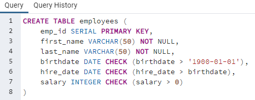
In the image above we use CHECK to make sure that the birthdate is greater than 1900, so only birthdates that are greater than that date will be allowed. Then I also CHECK hire_date greater than birthdate because hires can’t be below their birthdate. Last I made sure that the salary is greater than zero because a person’s salary can’t be 0.
Image example 2 (error):

The image above shows an error because the birthdate is lower than ‘1900-01-01’. I have put ‘1899-11-03’ to show that it violates the CHECK constraint. If you want to solve this error then you have to put a date higher than ‘1900-01-01’. For example, you can change ‘1899-11-03’ to '1949-11-03' and it will work because 1949 is higher than 1900.
CASE Statement
We use the CASE statement to execute SQL code when certain conditions are met. If you have learned other programming languages, it is similar to IF/ELSE statements.
Two main ways to use a CASE statement, either a general CASE or a CASE expression. Both methods produce the same results.
General syntax for general CASE:
CASE
WHEN condition1 THEN result1
WHEN condition2 THEN result2
ELSE some_other_result
END
Simple example with general CASE:
SELECT a,
CASE
WHEN a = 1 THEN ‘one’
WHEN a = 2 THEN ‘two’
ELSE ‘other’ AS label
END
FROM test;
The CASE expression syntax first evaluates an expression and then compares the result with each value in the WHEN clauses sequentially.
CASE expression syntax:
CASE expression
WHEN value1 THEN result1
WHEN value2 THEN result2
ELSE some_other_result
END
Our previous example, but with CASE expression:
SELECT a,
CASE a
WHEN 1 THEN ‘one’
WHEN 2 THEN ‘two’
ELSE ‘other’
END
FROM test;
Image example:

In the image above, I have made it so if customer_id is less than 100 it will return as ‘Premium’ then if a customer_id is between 100 and 200 it will return as ‘Plus’ then everything else will return as ‘Normal’.
* You can change name of the ‘case’ column to something else by adding AS after ‘END’
Image example for CASE expression:

You don’t have to write customer_id after WHEN.
COALESCE Function
The COALESCE Function accepts a limited number of arguments. It returns the first argument that is not null. If all arguments are null, the COALESCE function will return null.
COALESCE (arg_1,arg_2,…,arg_n)
Example syntax:
SELECT COALESCE (1,2); will return 1
SELECT COALESCE(NULL,2,3); will return 2
The function becomes useful when querying a table that has null values and substituting it with another value.
Example:
SELECT item,(price - COALESCE(discount,0))
AS final FROM table
* Remember the COALESCE function in mind when you encounter a table with null values that you want to perform operations on
CASE Operator
Lets you convert from one data type into another. Not every instance of data type can be CAST to another data type, it must be reasonable to convert the data, for example: ‘5’ to an integer will work, but ‘five’ to an integer will not.
*Useful for counting the lengths of integers since you can convert integers to strings and then use CHAR_LENGTH to count them.
Syntax:
SELECT CAST(‘5’ AS INTEGER)
PostgreSQL CAST operator:
SELECT ‘5’::INTEGER
* Keep in mind you can then use this in SELECT query with column name instead of single instance:
SELECT CAST(date AS TIMESTAMP) FROM table
NULLIF Function
The NULLIF function takes in 2 inputs and returns NULL if both are equal, otherwise, it returns the first argument passed
Example syntax:
NULLIF(arg1,arg2)
Example:
NULLIF(10,10) returns NULL
This becomes useful in cases where a NULL value had caused an error or has given you unwanted results.
VIEWS
Often times there are specific combinations of tables and conditions you find yourself using quite often in a project. Instead of performing the same query over and over again as a starting point, you can create a VIEW to quickly see this query with a simple call.
A view is a database object that is of a stored query. View does not store data physically, it stores the query.
Image example:

In the image above we have created a view of the INNER JOIN address and customer. You can name CREATE VIEW whatever you want, I just named it ‘customer_info’.
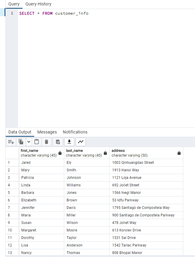
This is what it will return when you used CREATE VIEW. It is the same as using SELECT, INNER JOIN, and ON, but instead of writing out that long statement, we can just use CREATE VIEW and create a name for that long statement, in this case, I called it customer_info, so when I SELECT it FROM customr_info it outputs the same as when I was using INNER JOIN.
Overall you can expand on it such as adding HAVING statements or GROUP BY and so on. It helps you simplify things for complex queries.
If you want to add another column:

Use CREATE OR REPLACE VIEW to add another column. In this case, I want to add a district column, so I put the district on SELECT and the output is below
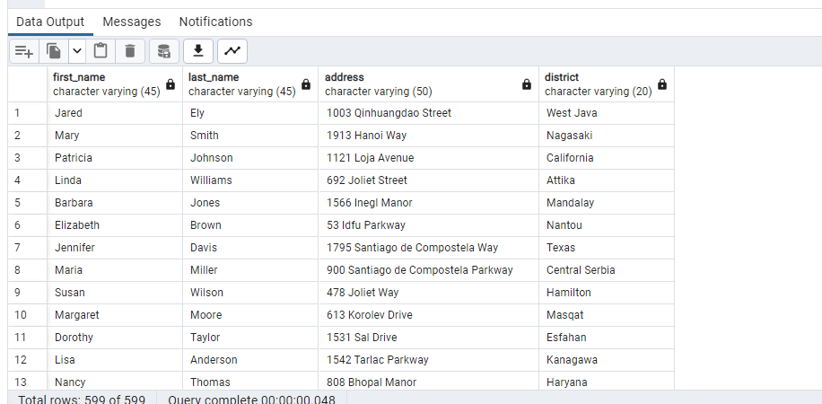
Use SELECT * FROM customer_info again and now you’ll see I have added a district column.
If you want to drop view use:
DROP VIEW IF EXISTS customer_info
If you want to change the table name:
ALTER VIEW customer_info RENAME to new_name
IMPORT and EXPORT
Not every data file will work, you must edit your file to be compatible with SQL.
* You must provide the 100% correct file path to your outside file, otherwise the import command will fail to find the file. Confirm you have the correct file path by checking the file’s location under its properties.
* The import command DOES NOT create a table for you. It assumes a table had already been created. So basically your .csv file must match the table you created.
You have reached the end of SQL. If you enjoyed this introduction and want to learn more about programming languages, software, data, and/or design then make sure to subscribe, so you don’t miss a post.