


Doing Data Analysis with SQL (Part One)
Learn how to use SQL specifically for data analysis or data science.

The Beginning of Data Analysis
What is Data Analysis?
Storing and collecting data for analysis is what a data analyst does. We would use many different tools such as Excel, R, Tableau, Python, SQL, etc, in order to understand data. Data analysis is part of communicating with data, discovering data, and interpreting data. The most common reason why we analyze data is to improve decision-making.
Analyzing data and finding the right number is just one part of what a data analyst does, but it’s also important to ask questions, stay curious, and understand why it works and the meaning behind it. It’s about understanding patterns, inconsistency, and discovering clues. Typically data arrives in a format that is ‘ugly’ and needs some improvement and decoration. No one would want to see an Excel sheet full of data presented to them, just like how no one wants to receive a long email.
Data analysis is used in human resources, marketing, logistics, UX design, sales, and more. It has led to massive job growth in related fields such as data science and data engineer. A bull market has happened in these fields.
Some organizations don’t do data analysis mainly because collecting, processing, and analyzing data takes time and money. Sometimes it’s because there isn’t a lot of data to generate or it may be illegal to gather data.
Being a great data analyst requires partnership. You can generate the right numbers, but if no one executes based on those numbers, it’s useless. Data is pretty much useless if no one uses them.
What is SQL?
SQL is what we would use to communicate with databases. SQL stands for Structured Query Language. SQL is used to manipulate, retrieve, and access data from objects in a database. A database can have one or more schemas. Objects used in data analysis are functions, tables, and views. Tables have fields, which contain data. Tables may have one or more indexes. Indexes are what help us find key values more easily. Views are stored queries that can be referenced. Functions allow us to store calculations or procedures and can be easily referenced in the query.
SQL has five sublanguages for handling different situations. You probably don’t need to know them, but it may come up. So here is the list:
DQL, or Data Query Language - is used for querying data (SELECT)
DDL, or Data Definition Language - is used to create and modify views, tables, and other objects in a database (CREATE, ALTER, DROP)
DCL, or Data Control Language - is used for access control (REVOKE, GRANT)
DML, or Data Manipulation Language - is used to act on data (UPDATE, INSERT, DELETE)
TCL, or Transaction Control Language - is used to control and manage transactions in a database (COMMIT, ROLLBACK)
SQL from another database may feel different, but the structure of the language is the same. SQL from MySQL, Oracle, and/or PostgreSQL may be a little different, but once you know SQL, you can work with all the different kinds of database software.
Data Workflow
When doing analysis, you want to begin with a question. Questions such as, how many sales did this product make, how many users did we acquire, etc. Once we got the question, we have to consider where we can find data, where will it be stored, the plan for analyzing data, and how we will present the data.
Data can be generated by a machine or by people. We can generate data by giving people a form to fill out. We can generate data from machines by having an application record a purchase, check out many clicks a website generated, and check out how many views this article is going to get when I publish it.
When we have gotten data, we can then move the data and store it for analysis. A data warehouse will combine all the data together and store it in a central repository.
The process for getting data into a data warehouse is called ETL, or extract, transform, load. Extract pulls data from the system. Transform changes the structure of the data such as cleaning the data or aggregating it. The load would put the data into the database. There are also source and target. The source is finding out where the data came from. Target is the destination.
 | Informatica")
Once the data is stored in the database, we can now perform analysis. We first perform analysis by exploring the data first, which is just to get familiar with it. After we’ve gotten familiar with the data, we can check the unique values in the data set. After we’ve checked the unique data, we can clean the data, which is fixing all the incorrect or missing data. Once we have finished cleaning, we can shape the data into rows and columns. Finally, we can analyze the data.
Presenting the data is what you would do last. Be sure to present it in charts, graphs, and insights because no one wants a bunch of SQL code handed to them. Also, you have to explain the results you’ve discovered.
Row-store databases
Row-store databases include PostgreSQL, MYSQL, SQL Server, etc. Row-store databases are good at transactions (INSERT, DELETE). They are widely used because of their low cost.
Tables will have a primary key, which is to prevent the database from creating the same record. There would also be a composite key, which contains two or more columns. This would make the row unique. For example, the columns customer_name, cutomer_age, and customer_purchase_date would make the row unique.
Column-store databases
Column-store databases store the values of columns together, rather than storing the values of rows. The most popular column-store databases include Snowflake, Google Cloud, and Amazon Redshift.
They are great at storing large volumes of data. They are more expensive than row-store databases, but if you want faster performance then choose this one.
Other databases
There are other databases such as the NoSQL database being the common one.
Preparing Data
Data preparation is easy when we have a data dictionary. A data dictionary is a document that contains descriptions of the columns, format, and fields. Most of the time we would not have a dictionary to help us. However, just because we weren’t given a dictionary doesn’t mean we can’t make one. Creating a data dictionary can help you and your team. Just keep the dictionary up to date and you can speed up your data process.

Data Types
Fields in the database table will have data types. The main types are numeric, logical, strings, and datetime. Here is a summary:
PS: Please read this summary on a laptop. It will look ugly and confusing on mobile.
Type:                                  Name:                                                      Description:

String                                CHAR/VARCHAR                                Holds strings
                                           TEXT                                                      Holds longer strings

Numeric                            INT/SMALLINT/BIGINT                   Holds integers
                                            FLOAT/DOUBLE/DECIMAL            Holds decimal numbers

Logical                               BOOLEAN                                            Holds TRUE or FALSE

Datetime                           DATETIME/TIMESTAMP                 Holds dates with times
                                            TIME                                                      Holds times
String data types will allow you to hold numbers, special characters, and letters.
Numeric data types will allow you to store positive and negative numbers. Decimals can also be stored.
The logical data type is BOOLEAN which has values of FALSE and TRUE.
The datetime types will store dates and times.
Structured and Unstructured
Unstructured data has no data models or data types. Things such as documents, images, videos, and emails are unstructured. Unstructured data is difficult to store efficiently. Therefore it is often stored outside of relational databases.
Semistructured data is between unstructured and structured data. Some unstructured data has a structure that we can use. For example, emails have email addresses that can be stored separately in a data model. Another example is audio files that may contain an artist's name, genre, and/or song name.
Structured data is stored in a column and each entity is represented as rows. You can easily query structured data using SQL.

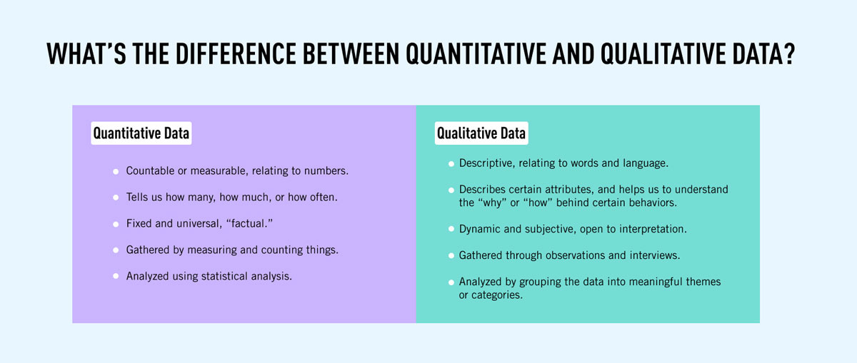
Quantitative and Qualitative Data
Quantitative data is numeric. It measures events, things, and people.
Qualitative data is usually a descriptive text that may contain words, opinions, and feelings.
First, Second, Third Party Data
First-party data is collected directly by you or by your organization. Because the data comes from your organization, it’s easy to communicate with people who have generated them and learn how the data is generated.
Second-party data is collected from vendors or another source. These are often automation tools, website trackers, and so forth. It is similar to first-party since it’s created by the organization, but the code that generates the data are external, and you would have little influence in adjusting the code if you want the code to produce something different.
Third-party data is often purchased or obtained from free sources. It lacks the proper frequency, quality, and format as the data isn’t collected specifically for your organization. Third-party data can be useful as it can provide demographics, trends, and spending patterns.
Sparse Data
Sparse data shows up as null values. Null, different from 0, is missing data. Sparse data can happen if there is an error in the software or in the early days of a product launch when there isn’t much data.
Sparse data can be a problem for analysis, so you should always find out where your data is sparse. You can exclude sparse data from the data set for the time being.
Profiling
When beginning analysis the first thing you should do is profiling. Look at how the data is arranged, the table name (in order to understand the topics), the column names, and the row names. Understand what the data is covering such is it marketing data, product data, sales data, and so forth. If possible understand how the data is generated, this makes it much easier.
Histograms and Frequencies
PS: You need some prior knowledge of SQL before reading on. Also, this is written in PostgreSQL.
The best way to know a data set is to check the frequency of values. It will show how many times a value occurs in the dataset.
SELECT column_name, COUNT(*) AS Quantity FROM table_name
GROUP BY 1;
A frequency plot is a great way to visualize the number of times it appears.
n-Tiles
n-tiles will allow us to calculate any percentile of the data set: such as the 78th percentile, 19th percentile, 34th percentile, and so forth.
NTILE(num_bins) OVER(PARTITION BY... ORDER BY...)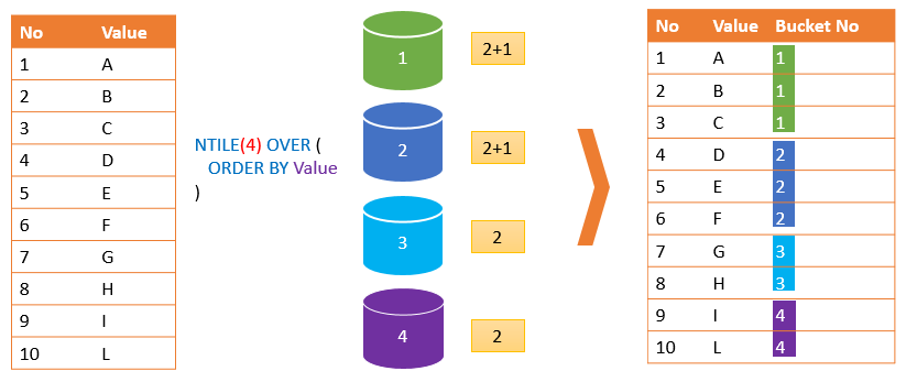
Example:

SELECT inventory_id, NTILE(10) OVER(ORDER BY inventory_id) as innn
FROM inventory
Note: The examples are from my dataset, so this would look different than yours, but the syntax should be the same.
There is also percent_rank which returns it as a percentile.
PERCENT_RANK() OVER (PARTITION BY... ORDER BY...)If you have a large data set, it can be expensive to compute since they sort all the rows. You can filter the data set to reduce the expense.
Data Quality
Data quality is crucial when having a good analysis. Just having good visualization isn’t good if the data is wrong. The saying is, “garbage in, garbage out” is true in this case. Putting garbage data in will only give you garbage data out.
Profiling is a way to prevent garbage data from going out.
Duplicates
Duplicates are where you have two or more rows that contain the same information. They can exist for many different reasons, such as a mistake made when entering data. JOINS can also result in duplicates.
You can find duplicates if all the columns are ordered:
SELECT column_a FROM table
ORDER BY 1
This will reveal if there are any data that are duplicates.
Here is a more systematic way to find duplicates:
SELECT COUNT(*) FROM
(
	SELECT column_a, column_b, column_c, column_d,
	COUNT(*) as name_you_choose
	FROM table
	GROUP BY 1
) a
WHERE name_you_choose > 1;
Example:
SELECT COUNT(*) FROM
(
SELECT inventory_id, film_id, store_id, last_update,
COUNT(*) as numbers
FROM inventory
GROUP BY 1
) a
WHERE numbers > 1;If the query returns 0, you are good.
It’s always a good idea to check why duplicates are happening, and if possible, fix it.
Deduplication with DISTINCT
The most popular way to remove duplicates is to use DISTINCT.
SELECT DISTINCT(column_a, column_b, column_c) FROM tableClean Data with CASE
CASE statements can be used to clean data. Even if the data was accurate, it would be more useful for analysis if values were grouped into categories.
CASE WHEN condition_1  THEN result_1
     WHEN condition_2  THEN result_2
     [WHEN ...]
     [ELSE else_result]
END
CASE statements can consider multiple columns and contain AND/OR logic. They can also be nested, but you can avoid this with AND/OR logic.
Cleaning with CASE statement works well if there is a short list of variations, you can find them all in the data, and the list isn’t expected to change. For a longer list, a lookup table can be a better option. The query will JOIN to the lookup table to get the cleaned data.
Type Conversions
Every field in a database is defined by a data type. When data is inserted into a table, values that aren’t of the field type are rejected. Strings can’t be inserted into integer fields, and booleans aren’t allowed in date fields.
Type conversions allow pieces of data with the appropriate format to be changed from one data type to another. One way to change data type is with the cast function, cast (input as data_type), or two colons, input :: data_type. For example, if we want to convert the integer 098765 to a string:
cast (098765 as varchar)


098765::varchar
Converting integers to strings can be useful in CASE statements when categorizing numeric values with some unbounded lower or upper value.
Function                                  Purpose
to_char                                     Converts other types to string
to_number                               Converts other types to numeric
to_date                                      Conerts othert types to dates, with specified date
to_timestamp                          Converts other types to dates, with specifed date and time
Sometimes database automatically converts a data type. For example, FLOAT and INT can be used together without changing the type. CHAR and VARCHAR values can be mixed.
Nulls
Nulls represent a field for which no data is collected or aren’t applicable for that row. There are a few ways to replace nulls: CASE statements, and the coalesce and nullif functions.
For CASE statements:
CASE WHEN city is null then 'Unknown' else city end

CASE WHEN city_id is null then 0 else city_id end
The coalesce function is more compact:
coalesce(city,'Unknown')

coalesce(city_id,0)
The nullif function compares two numbers and if they are not equal, it returns the first number. If they’re equal, the function returns null. For example, running this:
nullif(2,3)returns 2, whereas null is returned by:
nullif(2,2)Regardless of how you want to replace null, we need to consider them as targets for data cleaning.
Missing Data
Data can be missing for multiple reasons, each with its own implications for how you want to handle them.
We can often detect data by comparing values in two tables. For example, we can query the tables using a LEFT JOIN and add a WHERE condition:
SELECT distinct x.customer_id
FROM transactions x
LEFT JOIN customers y ON x.customer_id = y.customer_id
WHERE y.customer_id IS NULL
Missing data sometimes don’t always need to be fixed. It can reveal underlying system design or biases in the data collection process.
Records with missing fields can be filtered out, but we often want to keep them instead of making adjustments. We do have some options for in filling missing data, called imputation. This includes filling in the data with an average or median of the data set.
A common way to fill in missing data is with a constant value. It can be useful when the value is known for some records.
Another way is to fill in with a derived value, either a mathematical function on other columns or a CASE statement.
Missing values can also be filled with values from other rows in the data set.
Data can be missing for multiple reasons, and understanding why is important in deciding how to deal with it.
[End of Part One]